Linear Algebra
&
Engineering Mathematics 1
Week 11 - Probability
Probability Mass Functions vs Probability Discrete Functions
When we talk about random variables(RVs) in probability, they come in two types:
-
Discrete: Take on specific, separate values (like 0, 1, 2...).
- Continuous: Can take on any value within a range (like any real number between 0 and 6).

Probability Mass Functions vs Probability Discrete Functions
For discrete random variables we use a probability mass function (PMF) written as: \[ f_X(x) = Pr(X = x) \]
This means: "What is the probability that the random variable $X$ is exactly equal to the value $x$?"
Example: Tossing a fair die. 🎲 → $Pr(X=4)=\dfrac{1}{6}.$
To find the probability that $X$ lies in a range (like $2 ≤ X ≤ 4$), we add up the individual probabilities: \[ Pr(2\leq X \leq 4) = f_X(2) + f_X(3) + f_X(4). \]
Probability Mass Functions vs Probability Discrete Functions
For continuous random variables, we use a probability density function (PDF), denoted also by $f_X(x).$
Unlike discrete variables, we cannot calculate probabilities at exact points:
For all real numbers $a$: $\;Pr(X = a) = 0.$
Instead, we calculate probabilities over intervals using integration: \[ Pr(a\lt X\lt b) = \int_a^bf_X(x)\,dx \]
This integral represents the area under the curve of the PDF between $a$ and $b,$ which gives the probability that $X$ lies within that range.
Summary: Discrete vs Continuous Random Variables
| Random Variable Type | Function Name | Notation | Probability for Range |
|---|---|---|---|
| Discrete | PMF (mass) | \( f_X(x) \) | \( \ds \Pr(X \in A) = \sum_{x \in A} f_X(x) \) |
| Continuous | PDF (density) | \( f_X(x) \) | \( \ds\Pr(a < X < b) = \int_a^b f_X(x)\,dx \) |
Example: Throwing a fair die 🎲
The probability that any of one of the six sides of a fair die 🎲 lands uppermost when thrown is 1/6. This can be represented be represented mathematically as: \[ P(X = x) = \frac{1}{6}, \hspace{0.3 cm} x = 1, 2, \ldots, 6. \]
- \(X\) represents the random variable describing the side that lands uppermost.
- \(x\) represents the possible values \(X\) can take.

Cumulative Density Function (CDF)
The cumulative density function (CDF) of a random variable is the probability that the random variable takes a value less than or equal to a specified value, $x$: \[ F(x) = Pr(X \leq x) \]
| $X$ | 1 | 2 | 3 | 4 | 5 | 6 |
| $f_X(x)$ | $\dfrac{1}{6}$ | $\dfrac{1}{6}$ | $\dfrac{1}{6}$ | $\dfrac{1}{6}$ | $\dfrac{1}{6}$ | $\dfrac{1}{6}$ |
| $F(x)$ | $\dfrac{1}{6}$ | $\dfrac{2}{6}$ | $\dfrac{3}{6}$ | $\dfrac{4}{6}$ | $\dfrac{5}{6}$ | $\dfrac{6}{6}$ |
👆 Throwing a die 🎲
Cumulative Density Function (CDF)
|
$F(x) = Pr(X \leq x)$
👆 Throwing a die 🎲 |


|
Cumulative Density Function (CDF)


The uniform distribution (Discrete & Continuous)
|
|
|
|
|
|
Checkpoint: Problem 1
Let $X$ denote the random variable that measures the sum of the sides that come up when rolling two fair dice 🎲🎲 simultaneously.
- Write down the sample space of $X$ (what are possible values of $X$?)
- Write down the probability mass function (PMF) of $X,$ in a tabular form.
- Use the PMF in part 2 to write down the cumulative distribution function (CDF) of $X$ in a tabular form.
Checkpoint: Problem 2
The continuous random variable $Y$ is uniformly distributed on the interval $(1,2).$
- Write down the probability density function (PDF) of $Y.$
- Sketch the graph of the pdf of $Y.$
- By thinking about the geometry of the PDF, write down a formula for the CDF of $Y$ (you do not have to do integration to work this out). Sketch this CDF.
Checkpoint: Problem 2
The continuous random variable $Y$ is uniformly distributed on the interval $(1,2).$
- Write down the probability density function (PDF) of $Y.$
- Sketch the graph of the pdf of $Y.$
-
By thinking about the geometry of the PDF,
write down a formula for the CDF of $Y$
(you do not have to do integration to work this out). Sketch this CDF.
Bayes' Theorem
Suppose we have two events: $A$ and $B.$ The probability of both occurring simultaneously is
1. $P(A \text{ and } B) = P\left(A \,|\, B\right)P(B)$
2. $P(A \text{ and } B) = P\left(B \,|\, A\right)P(A)$
This implies $\,P\left(A \,|\, B\right)P(B) = P\left(B \,|\, A\right)P(A)$
⭐️ $P\left(A \,|\, B\right)= \dfrac{P\left(B \,|\, A\right)P(A)}{P(B)}$ ⭐️
Bayes' Theorem
⭐️ $P\left(A \,|\, B\right)= \dfrac{P\left(B \,|\, A\right)P(A)}{P(B)}$ ⭐️
Since $P(B) =$ $\, P\left(B \,|\, A\right)P(A) $ $\,+$ $\, P\left(B \,|\, A'\right)P(A'),$ then
$P\left(A \,|\, B\right)= \dfrac{P\left(B \,|\, A\right)P(A)}{P\left(B \,|\, A\right)P(A) + P\left(B \,|\, A'\right)P(A')}$
Example 👉 Medical Diagnosis
The Normal Distribution
$ \large f_X(x; \mu, \sigma) =\ds \frac{1}{\sigma \sqrt{2\pi}} e^{-\frac{1}{2} \left( \frac{x - \mu}{\sigma} \right)^2}, $
$x \in \R,\, \mu \in \R, \sigma > 0,$

The Normal Distribution
$ \large N\left(\mu, \sigma^2\right) =\ds \frac{1}{\sigma \sqrt{2\pi}} e^{-\frac{1}{2} \left( \frac{x - \mu}{\sigma} \right)^2}$
We write $X\sim N\left(\mu, \sigma^2\right)$:
$X$ is normally distributed with mean $\mu$ and variance $\sigma^2.$
The Normal Distribution
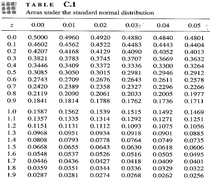
Areas under the Standard Normal Distribution
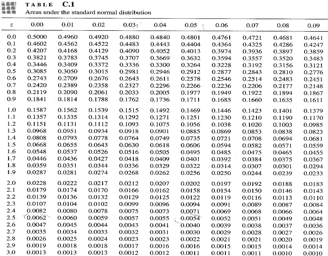
Areas under the Standard Normal Distribution
|
👈 |
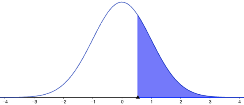
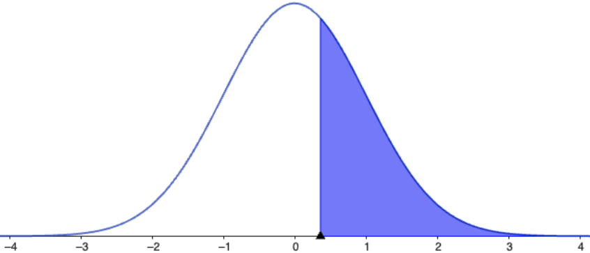
$Z\sim N(0,1)$ $P(Z\gt a)$ |
Areas under the Standard Normal Distribution
Example 1: $Z \sim N(0,1).$ Find $P(Z\gt 1.52)$
Areas under the Standard Normal Distribution
Example 2: $Z \sim N(0,1).$ Find $P(0 \lt Z \lt 1.52)$
Areas under the Standard Normal Distribution
Exercise 1: Find $P( Z \lt -1.93)\qquad \;\,\,$
Exercise 2: Find $P( -1.52 \lt Z \lt 1.52)$
Example: How to apply the transformation $Z = \frac{x-\mu}{\sigma}$
Many university students do some part-time work to supplement their allowances. In a study on students' wages earned from part-time work, it was found that their hourly wages are normally distributed with mean, $\mu = \$ 16.20$ and standard deviation $\sigma = \$3.$ Find the proportion of students who do part-time work and earn more than $25.00 per hour.
Probability distributions
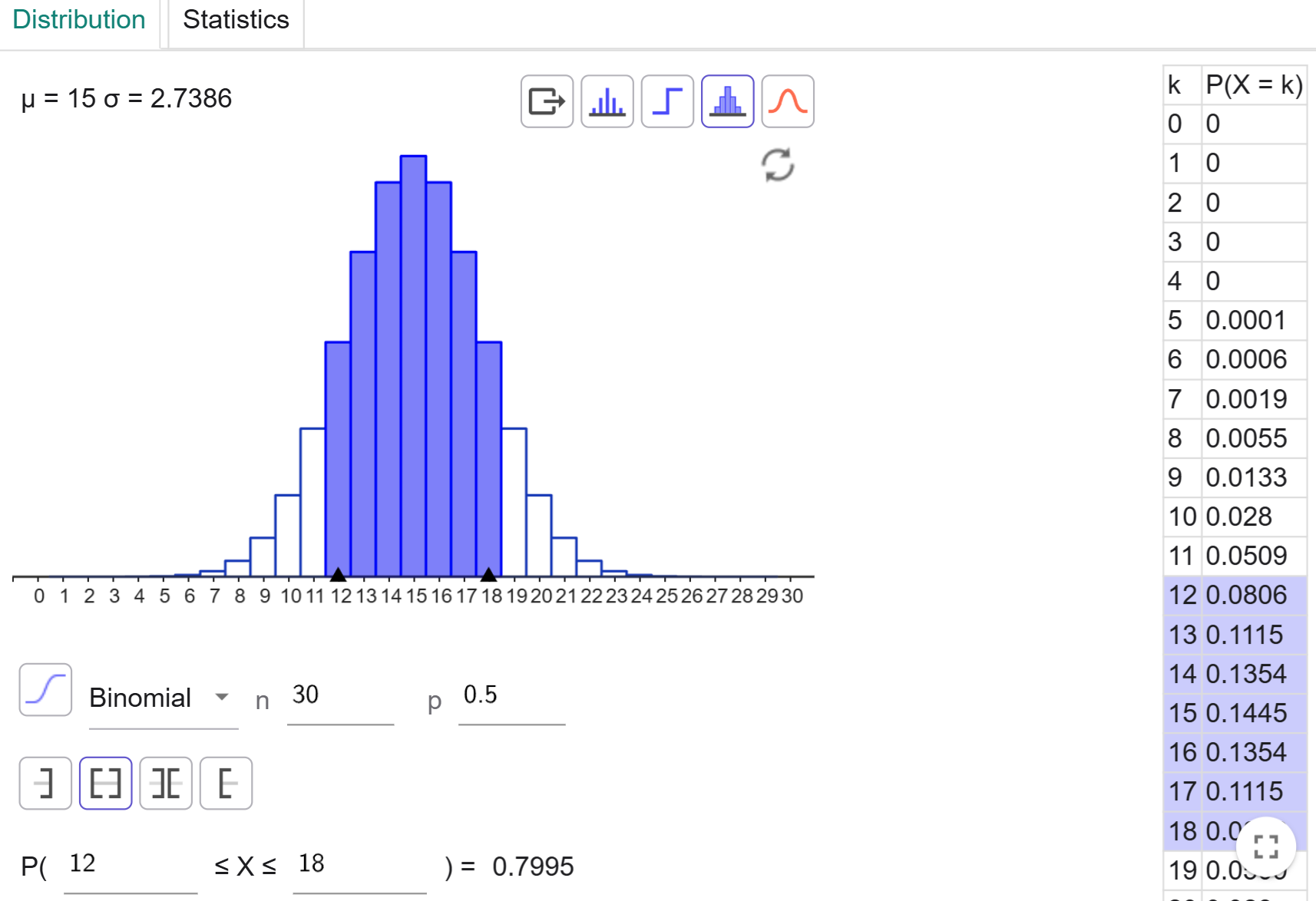
$P(X=k)$ $=$ $^nC_k $ $p^{\,k}$ $(1-p)^{n-k}$
Probability distributions
| Normal distribution: \[ N\left(\mu, \sigma^2\right) =\ds \frac{1}{\sigma \sqrt{2\pi}} e^{-\frac{1}{2} \left( \frac{x - \mu}{\sigma} \right)^2} \] |
|
| Poisson distribution: \[ P\left(X=k\right) =\ds \frac{e^{-\lambda }\lambda^k}{k!}, \;k = 0, 1, \ldots, \lambda \gt 0 \] | 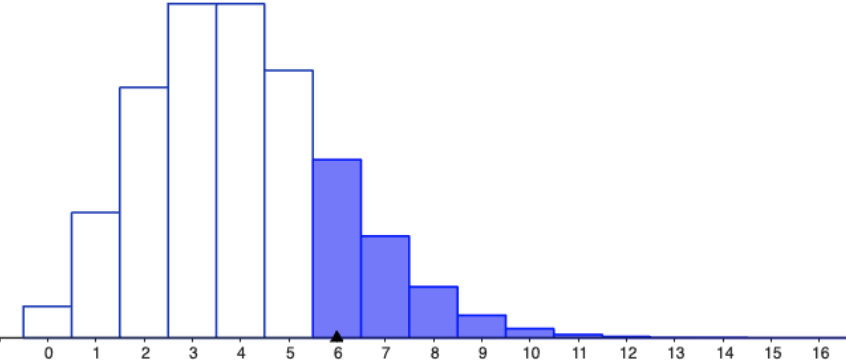 |
| Exponential distribution: \[ f_X(x) =\ds \left\{ \begin{array}{rl} \lambda e^{-\lambda x}, & x\geq 0\\ 0, & \text{otherwise} \end{array} \right. \] | 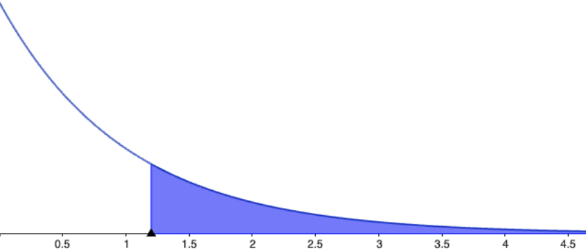 |
Key properties of the Poisson distribution
\[ P\left(X=k\right) =\ds \frac{e^{-\lambda }\lambda^k}{k!} \]
- $k$ is the number of occurrences ($k = 0, 1, \ldots$ ).
- $\lambda $ is a positive parameter ($\lambda \gt 0$) known as the rate of occurrence.
- $E(X) = \lambda .$
-
If $X_1, X_2,\ldots , X_n$ are independent Poisson random variables with
parameters $\lambda_1,\lambda_2,\ldots,\lambda_n,$ respectively,
then
$X =\ds \sum_{k=1}^{n}X_i $ $\ds \sim \text{Poisson}\left(\sum_{k=1}^{n}\lambda\right)$
Probability distributions
Checkpoint: Bank Tellers Problem
The manager of a bank branch supervises three tellers. The number of customers each teller can serve in a 10-minute period follows a Poisson distribution, but with different rates: Teller A serves customers at a rate of 2 per 10 minutes, Teller B at a rate of 3 per 10 minutes, and Teller C at a rate of 4 per 10 minutes.
- If the tellers serve customers independently of each other, write down the probability distribution of the total number of customers this branch can serve in a 10 minute period when fully staffed.
- How many customers would you expect this branch to serve in a 10 minute period if fully staffed?
- Calculate the probability that the total number of customers served in a 10 minute period at this branch exceeds 5 people, when fully staffed.
Checkpoint: Bank Tellers Problem
- If the tellers serve customers independently of each other, write down the probability distribution of the total number of customers this branch can serve in a 10 minute period when fully staffed.
Let \( X_A \sim \text{Poisson}(2) ,\) \( X_B \sim \text{Poisson}(3),\) and \( X_C \sim \text{Poisson}(4) ,\)
All independent.
The total number of customers served is:
$ X = X_A + X_B + X_C $ $\ds \sim \text{Poisson}(2 + 3 + 4) = \text{Poisson}(9)$
Checkpoint: Bank Tellers Problem
- How many customers would you expect this branch to serve in a 10 minute period if fully staffed?
\( X_A \sim \text{Poisson}(2) ,\)
\( X_B \sim \text{Poisson}(3),\)
\( X_C \sim \text{Poisson}(4) ,\) independent.
The expected value of a Poisson distribution
is its rate parameter \( \lambda \).
Thus
$ E(X) $ $= 2 + 3 + 4 =9$
Checkpoint: Bank Tellers Problem
- Calculate the probability that the total number of customers served in a 10 minute period at this branch exceeds 5 people, when fully staffed.
We want to compute \( P(X > 5) \)
where \( X \sim \text{Poisson}(9) .\)
Use the complement rule:
$ \quad P(X > 5) = 1 - P(X \leq 5) $ $= 1 - \ds \sum_{k=0}^{5}P\left(X=k\right) $
$ \qquad \qquad = 1 - \left[ \ds \frac{e^{-9}9^{0}}{0!} + \frac{e^{-9}9^{1}}{1!} + \frac{e^{-9}9^{2}}{2!} + \frac{e^{-9}9^{3}}{3!} + \frac{e^{-9}9^{4}}{4!} + \frac{e^{-9}9^{5}}{5!}\right] $
Key properties of the Exponential distribution
\[ f_{X}(x)=\ds \left\{ \begin{array}{rl} \lambda e^{-\lambda x}, & x\geq 0\\ 0, & \text{otherwise} \end{array} \right. \]
- We write $X\sim Exp(\lambda).$
-
The CDF of $X\sim Exp(\lambda)$ is
$\quad P(X\lt x)=$ $\ds F_X(x) =\ds \left\{ \begin{array}{rl} 1-e^{-\lambda x}, & x\geq 0\\ 0, & \text{otherwise} \end{array} \right.$
- $E(X) = \dfrac{1}{\lambda} $ and $\text{Var}(X) = \dfrac{1}{\lambda^2}.$
- If $X\sim Exp(\lambda),$ then \[ \qquad \qquad P\left(X\gt s+t \,|\, X\gt t\right) = P\left( X\gt s\right). \]