Quantitative Reasoning
1015SCG
Lecture 5

Functions
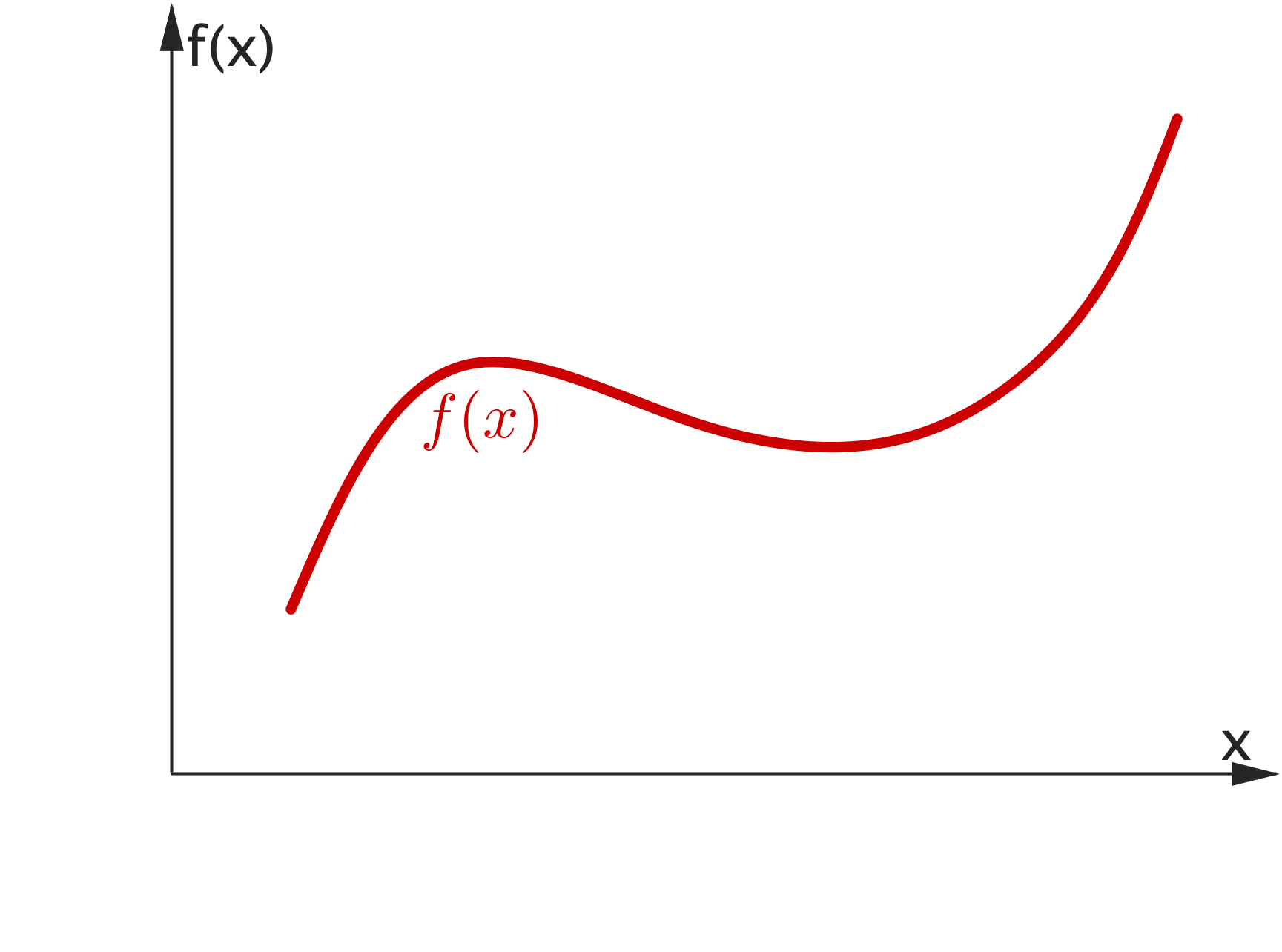
What is a function? 🤔
Function Machine
Functions
What is a function? 🤔
A function is a rule that associates a unique output to each input.
Definition: A function assigns to each element of $X$ (set of numbers) exactly one element of $Y$ (also a set of numbers).
The set $X$ is called the domain of the function and the set $Y$ is called the range of the function.
Functions
$f(x) = 3x+2$
|
$f(3) = 3(3)+2$ $\quad\;\;\,\, =9 + 2$ $\quad\;\;\,\, =11$ |
$f(-5) = 3(-5)+2$ $\quad\;\;\,\, = -15+2$ $\quad\;\;\,\, = -13$ |
Functions
$f(x) = x^2-2x+4$
|
$f(-4) = (-4)^2-2(-4)+4$ $\qquad\,\, =16 + 8+4$ $\qquad\,\,=28$ |
$f(2a) = (2a)^2-2(2a)+4$ $\qquad\,\,= 4a^2-4a+4$
|
Functions
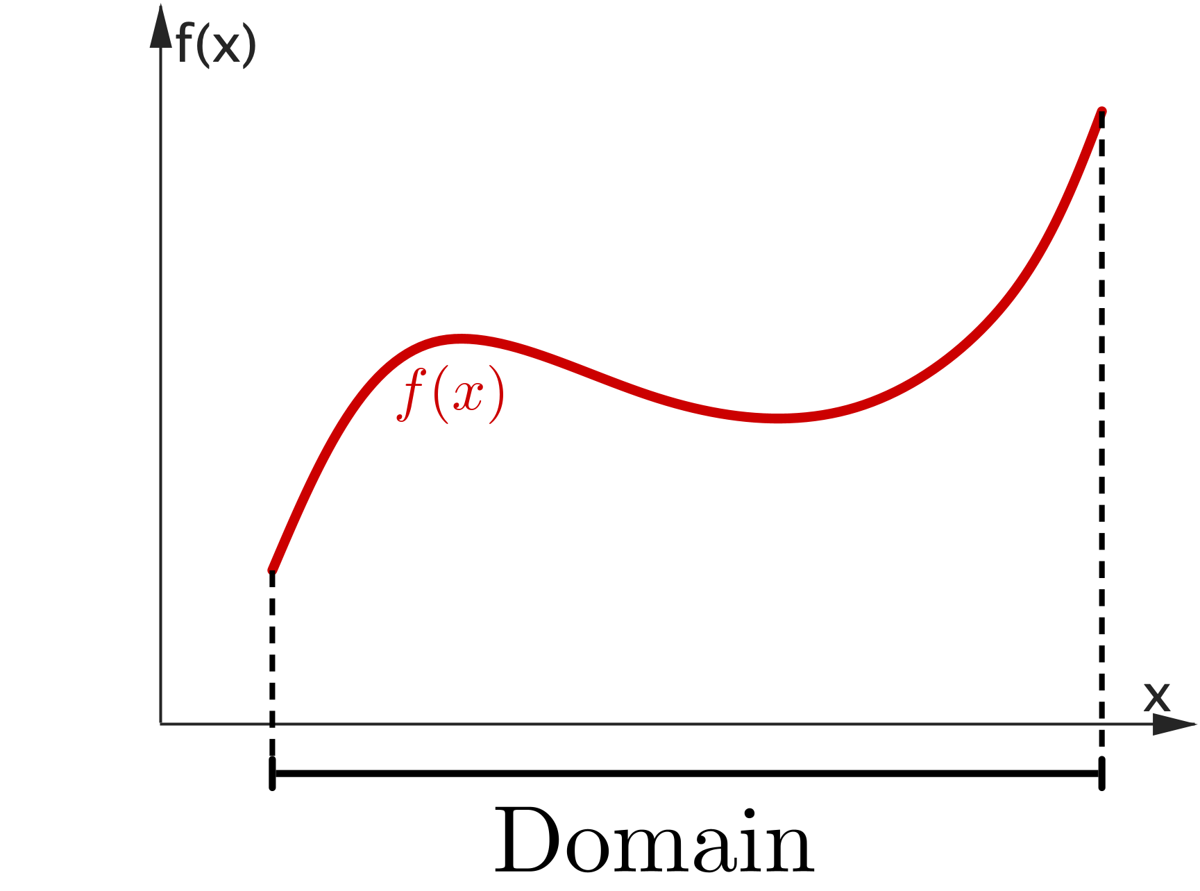
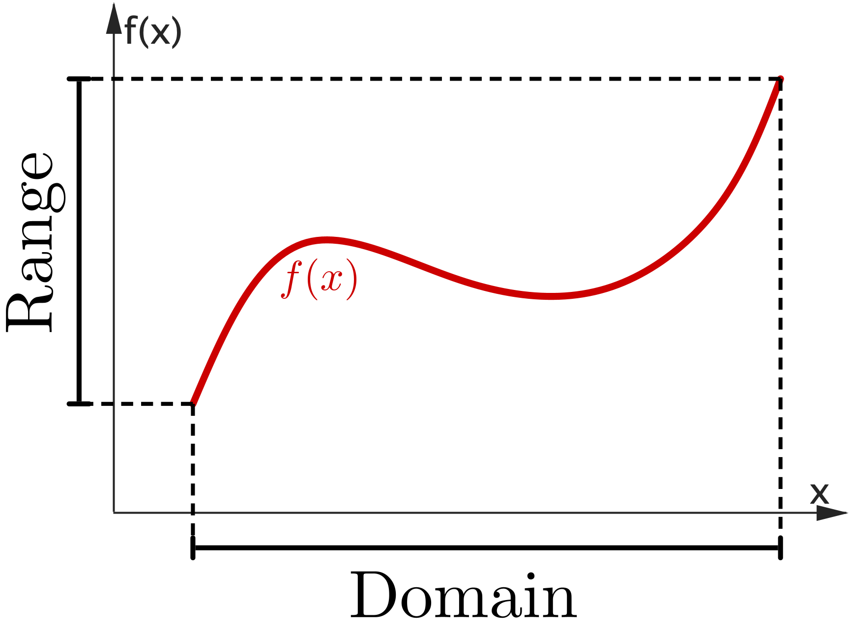
|
The domain of $f(x)$ is the set of all possible values of $x$ for which the function is defined (i.e. all the values of $x$ that can be used with the function). The range of $f (x)$ is the set of all possible values that can be returned by the function. |
Functions
Consider the function $f(x)= \dfrac{1}{x-5}$

|
$f(0) = \dfrac{1}{(0)-5}$ $=-\dfrac{1}{5}$ $f(-2) = \dfrac{1}{(-2)-5}$ $=-\dfrac{1}{7}$ $f(9) = \dfrac{1}{(9)-5}$ $=\dfrac{1}{4}$ $f(5) = \,$ Not possible! 1/0! Domain: All real values of $x,$ except $x=5.$ Range: All real values except $0.$ |
Elementary functions
Polynomials

Exponentials & Logarithms

$f(x) = 2^x,\;\;$ $g(x)=e^x$ |

$f(x) = \ln(x),\;\;$ $g(x)=\log_{2}(x)$ |
|---|
Recall: Index Laws
|
Extra:
$\large a^{\frac{1}{n}} = \sqrt[n]{a}$ |
Recall: Logarithm Laws
- Product Law: $\;\log_a\left(M\times N\right)$ $=\log_a M + \log_a N$
- Quotient Law: $\;\log_a\left(\dfrac{M}{N}\right)$ $=\log_a M - \log_a N$
- Power Law: $\;\log_a\left(N^p\right)$ $= p \times \log_a (N)$
- Trivial identities: $\;\log_a(a) = 1\;$ and $\;\log_a(1) = 0 $
These rules work for any base \( a > 0 ,\) \( a \ne 1 .\)
Recall: Change of Base Rule
\[ \large \log_b (N) = \frac{\log_a (N)}{\log_a (b)} \] where \( a \) can be 10 (common log) or \( e \) (natural log).
Example: $\log_2 10$ $ =\dfrac{\log_{10} 10}{\log_{10} 2} $ $ \approx \dfrac{1}{0.3010}$ $\approx 3.32$
Why do we need logarithms anyway?

Why do we need logarithms anyway?
Imagine we are living in 1823 and we need to compute \[ x=\sqrt[3]{\frac{493.8\times \left(23.67\right)^2}{5.104}}. \]
😬 ❌ 🖥️
Why did you need to make such
calculation?
🧭 🗺️ 🌌 🔭
Why do we need logarithms anyway?
Imagine we are living in 1823 and we need to compute $ \ds x=\sqrt[3]{\frac{493.8\times \left(23.67\right)^2}{5.104}}. $
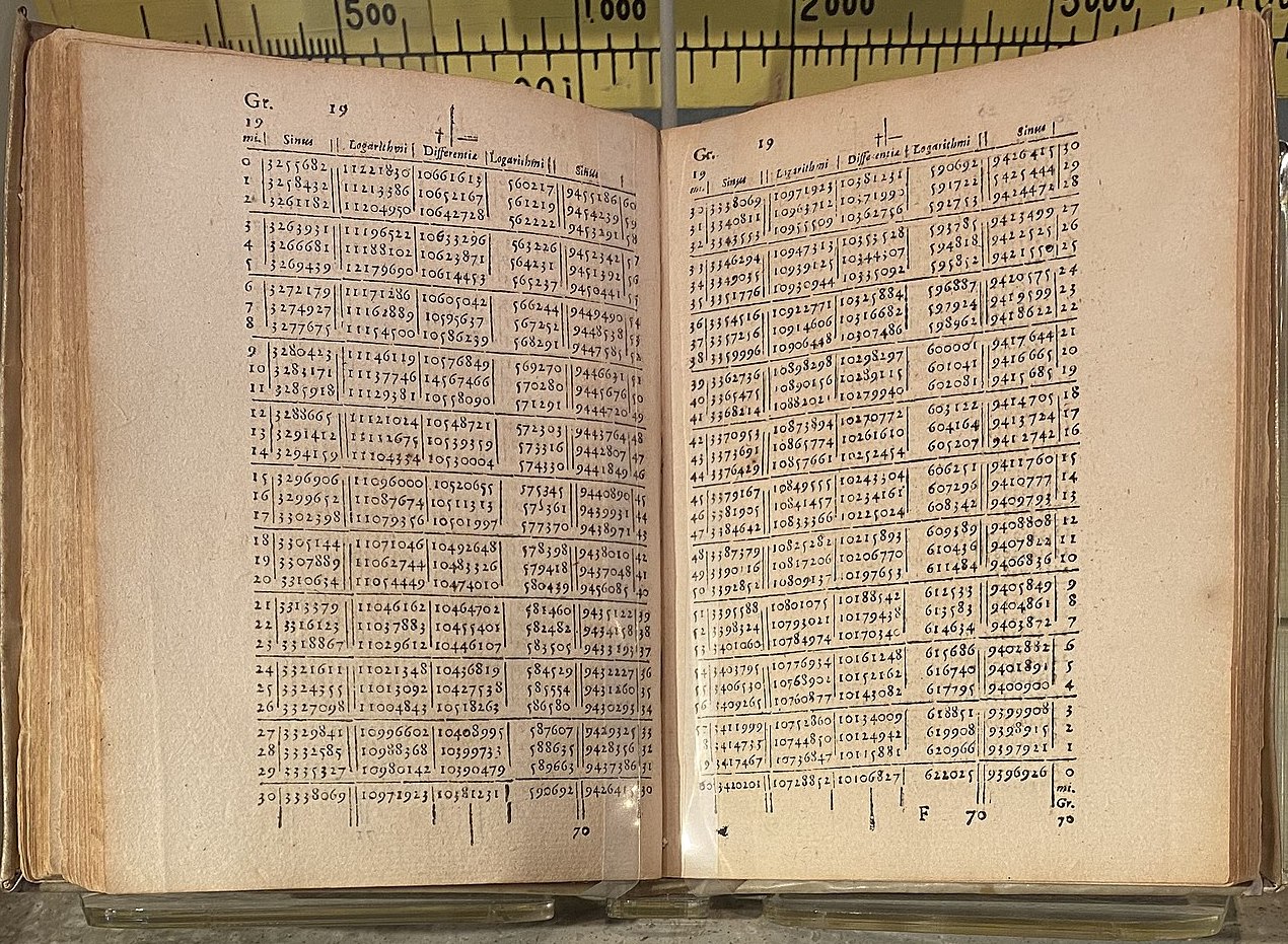
Why do we need logarithms anyway?
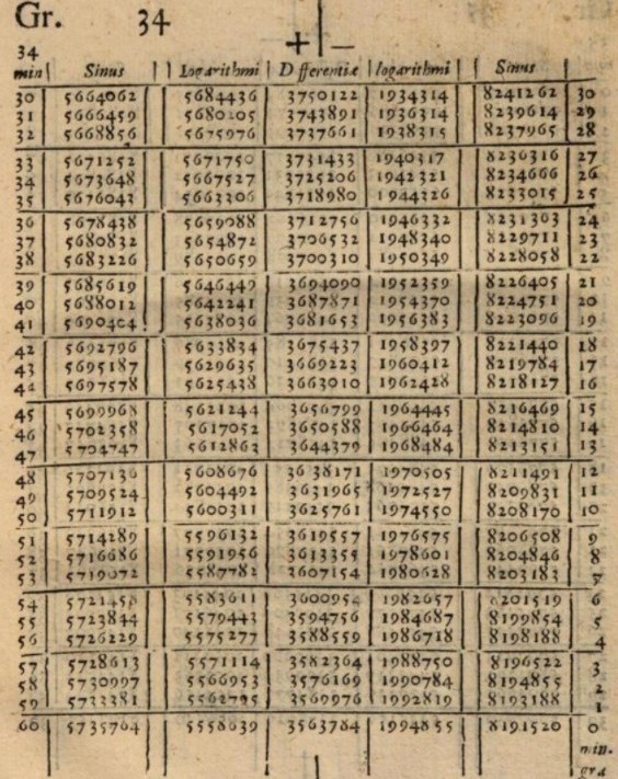
So, how do we compute $ \ds x=\sqrt[3]{\frac{493.8\times \left(23.67\right)^2}{5.104}}. $
We can write $\,\ds x=\left(\frac{493.8\times \left(23.67\right)^2}{5.104}\right)^{1/3}$
Using the properties of the logarithms, we have
$ \ds \log x=\frac{1}{3}\bigg(\log (493.8)+2\log (23.67)-\log (5.104)\bigg) $
Why do we need logarithms anyway?
$ \ds \log x=\frac{1}{3}\bigg(\log (493.8)+2\log (23.67)-\log (5.104)\bigg) $
|
Then we find these values using the logarithmic tables. 👉 $\;x\approx 37.84$ |
|
Why do we need logarithms anyway?
Hence, if $\; \ds x = \sqrt{\frac{493.8\times (23.67)^2}{5.104}}, $ we have that $\,x\approx 37.84$

Why do we need logarithms anyway?
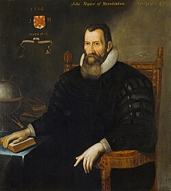
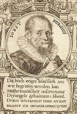
Logarithms exists thanks to John Napier and Jost Bürgi who discovered independently at the beginning of the XVII century.
|
|
Why do we need logarithms anyway?
Since nothing is more tedious, fellow mathematicians, in the practice of the mathematical arts, than the great delays suffered in the tedium of lengthy multiplications and divisions, the finding of ratios, and in the extraction of square and cube roots- and in which not only is there the time delay to be considered, but also the annoyance of the many slippery errors that can arise.
John Napier (1614)
Trigonometric functions
Trigonometric functions

Recall: sin / cos / tan ratios
|
\(\sin\left(\theta \right) = \dfrac{\text{opposite}}{\text{hypotenuse}}\) \(\cos\left(\theta \right) = \dfrac{\text{adjacent}}{\text{hypotenuse}}\) \(\tan\left(\theta \right) = \dfrac{\text{opposite}}{\text{adjacent}}\) |


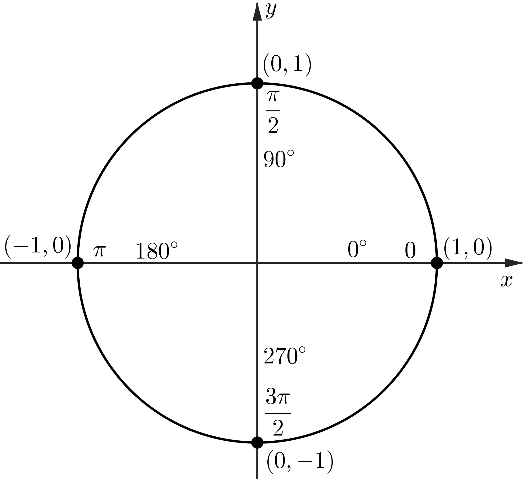
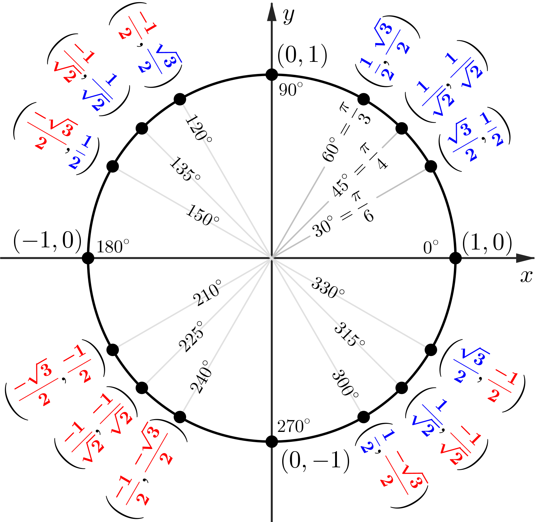
The Unit Circle
The Unit Circle
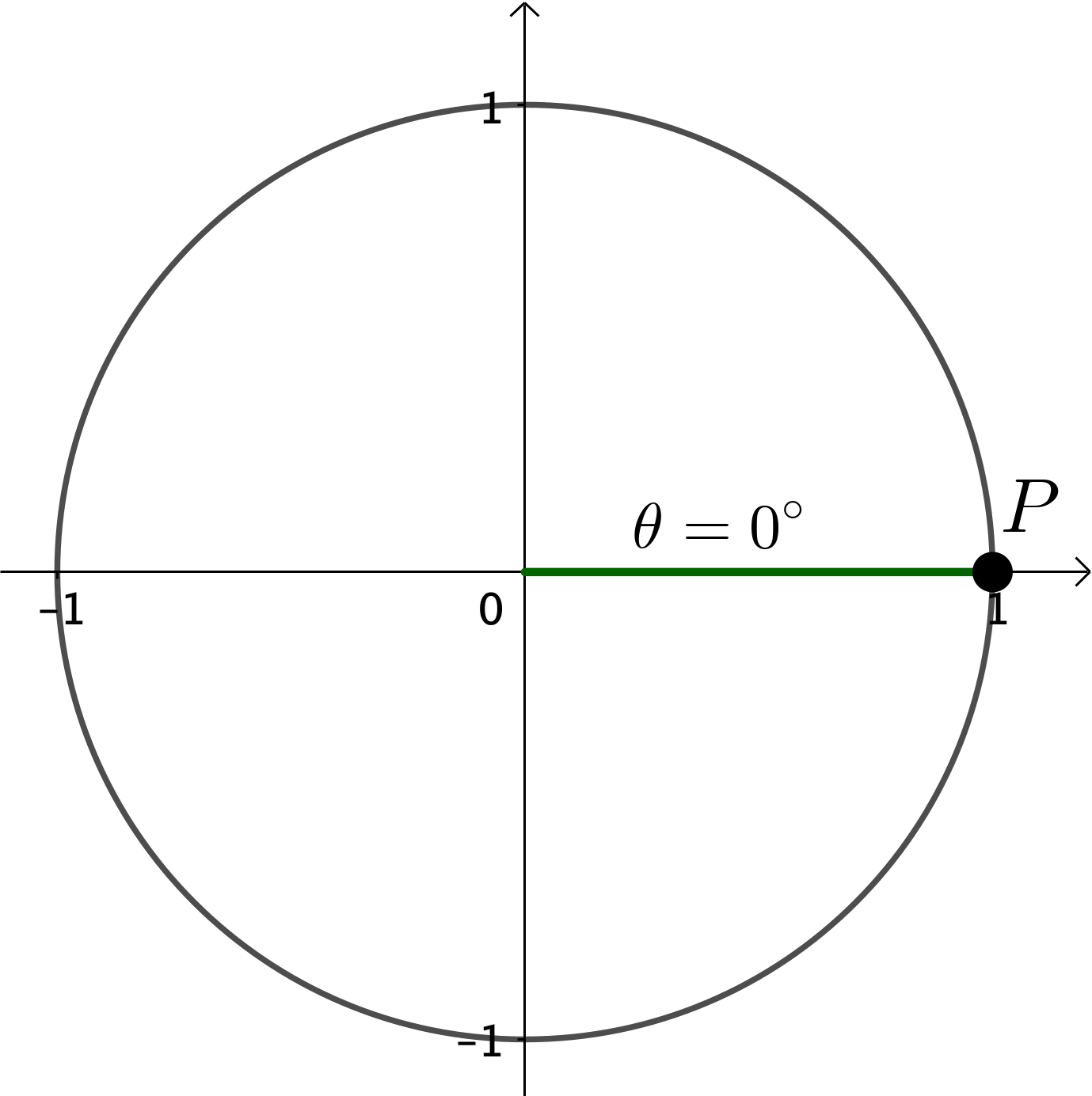
|
\(P = \left(\cos \theta, \sin \theta\right)\) \(\;\;\; = \left(\cos 0^{\circ}, \sin 0^{\circ}\right)\) \(\;\;\; = \left(1, 0\right)\) |
The Unit Circle
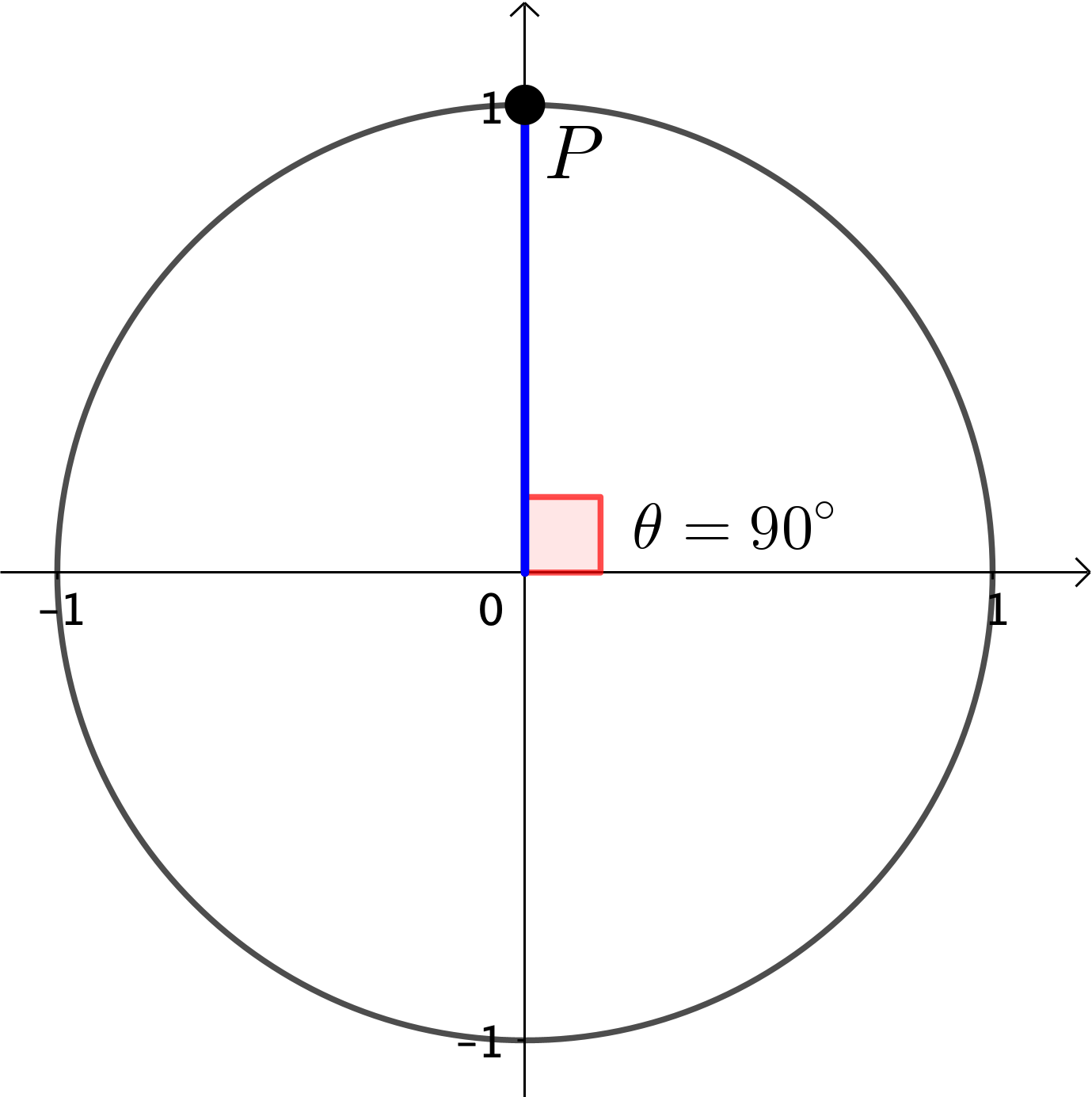
|
\(P = \left(\cos \theta, \sin \theta\right)\) \(\;\;\; = \left(\cos 90^{\circ}, \sin 90^{\circ}\right)\) \(\;\;\; = \left(0, 1\right)\) |
The Unit Circle
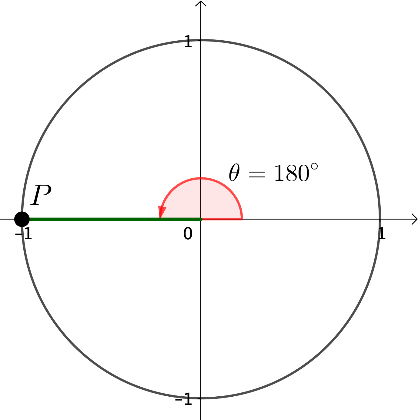
|
\(P = \left(\cos \theta, \sin \theta\right)\) \(\;\;\; = \left(\cos 180^{\circ}, \sin 180^{\circ}\right)\) \(\;\;\; = \left(-1, 0\right)\) |
The Unit Circle
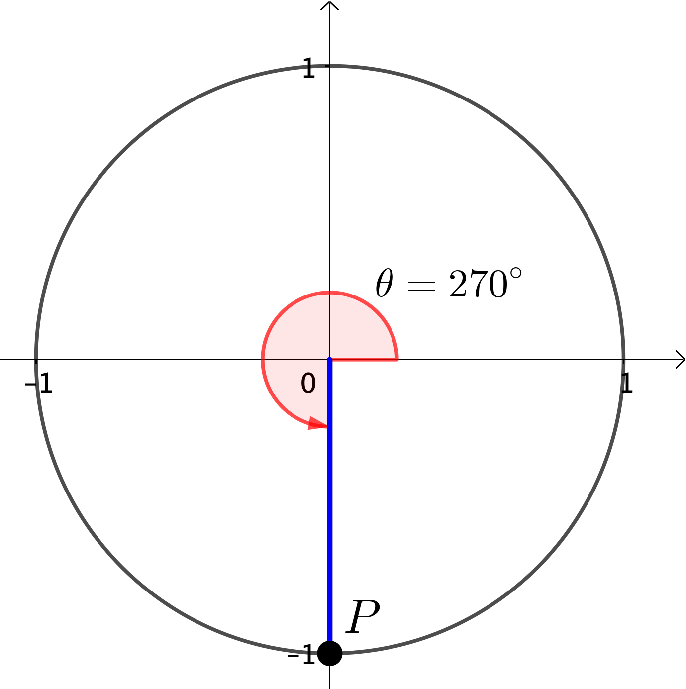
|
\(P = \left(\cos \theta, \sin \theta\right)\) \(\;\;\; = \left(\cos 270^{\circ}, \sin 270^{\circ}\right)\) \(\;\;\; = \left(0, -1\right)\) |
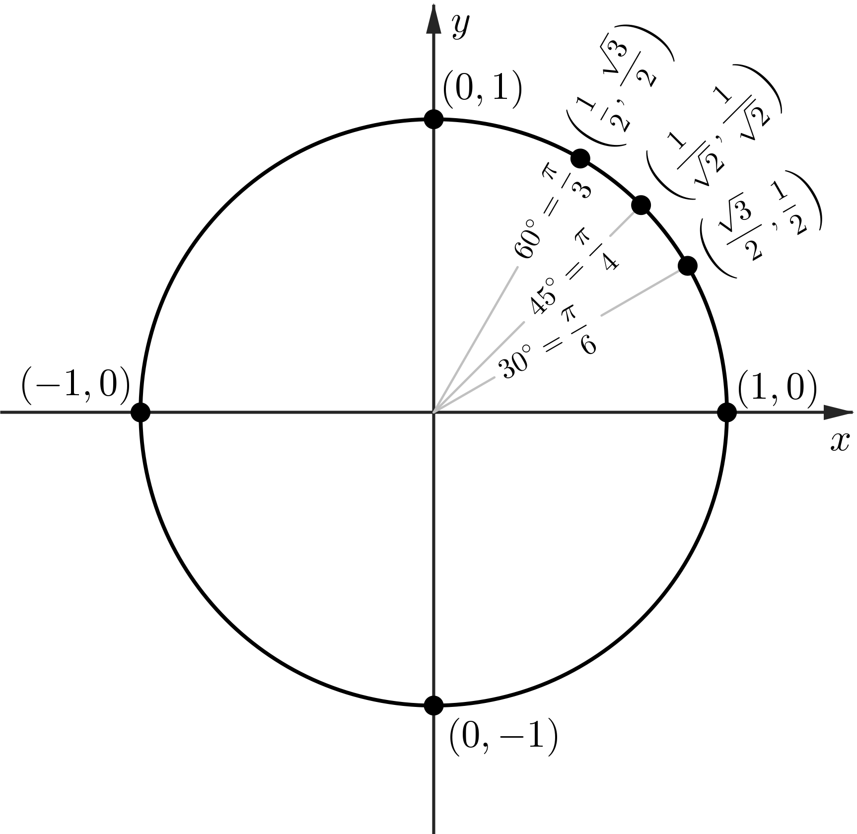
The Unit Circle: sin and cos at $30^\circ$ or $\pi/6$
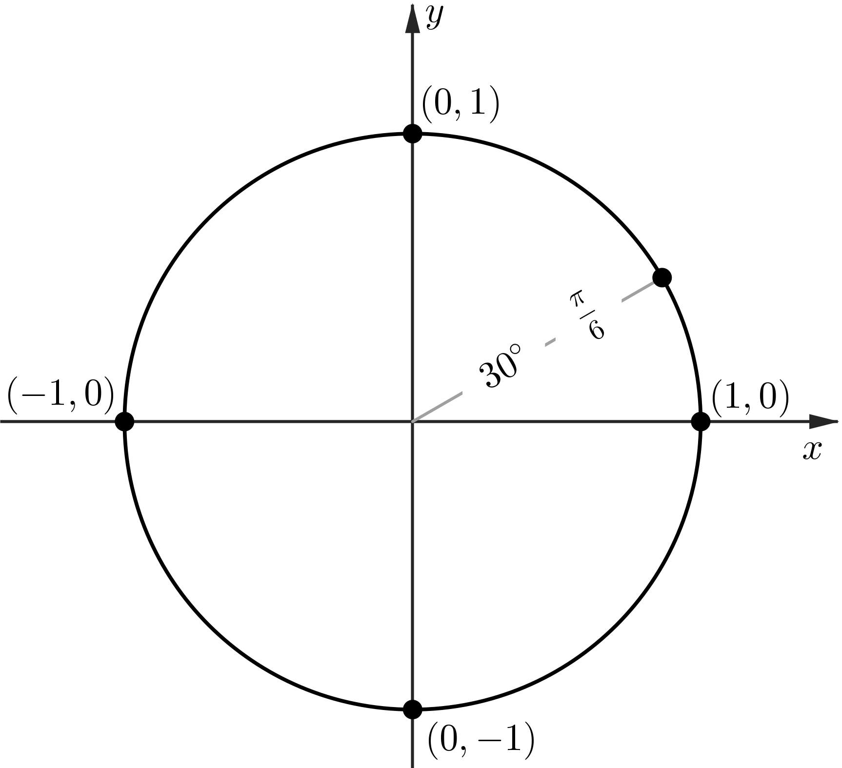
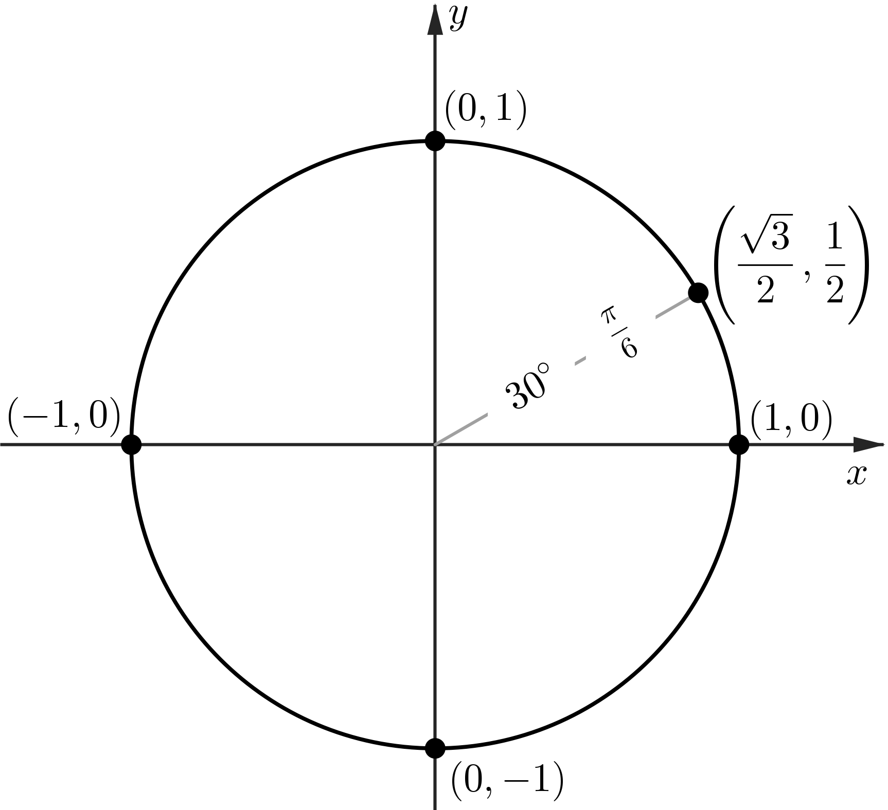
|
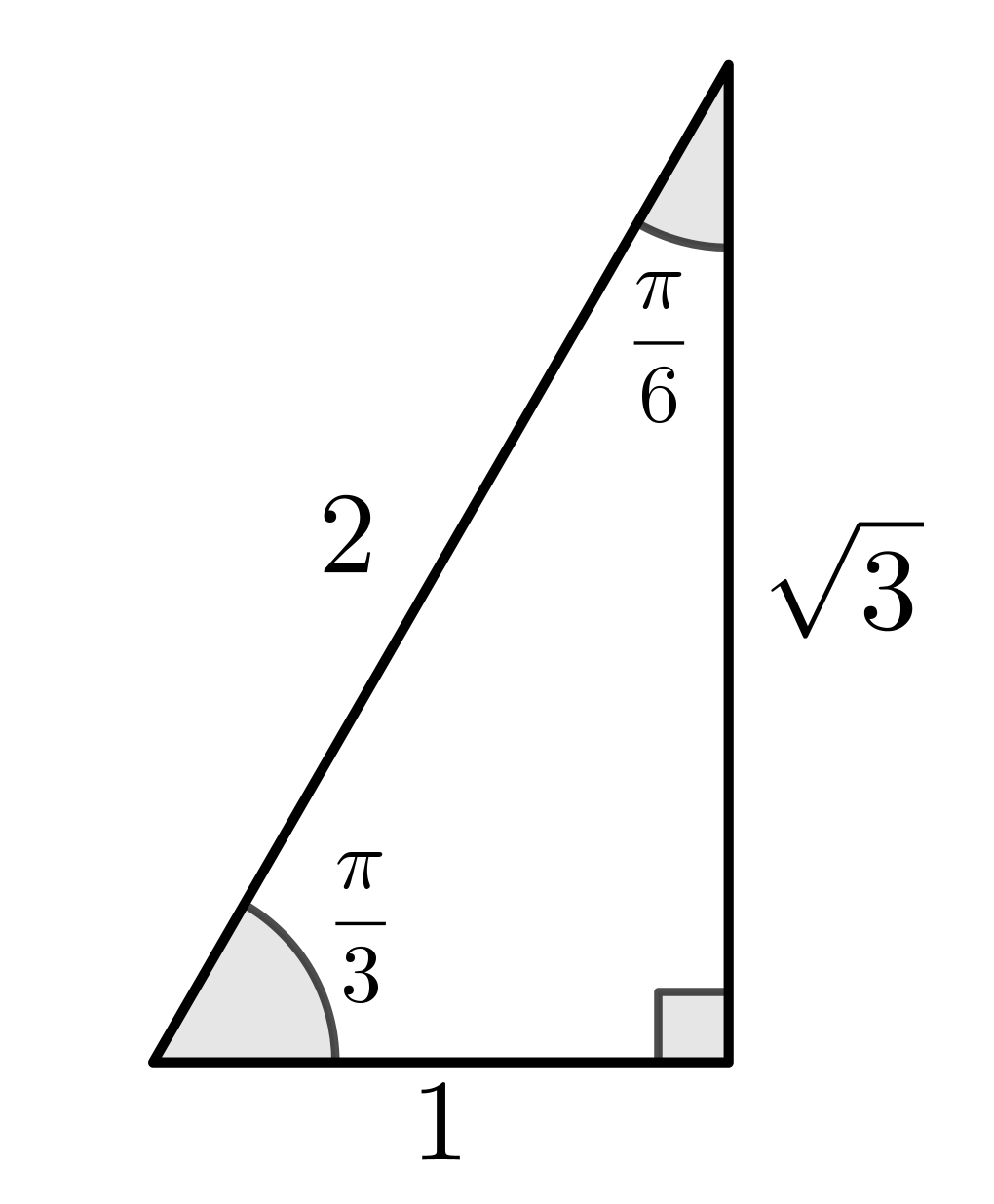
|
The Unit Circle: sin and cos at $45^\circ$ or $\pi/4$
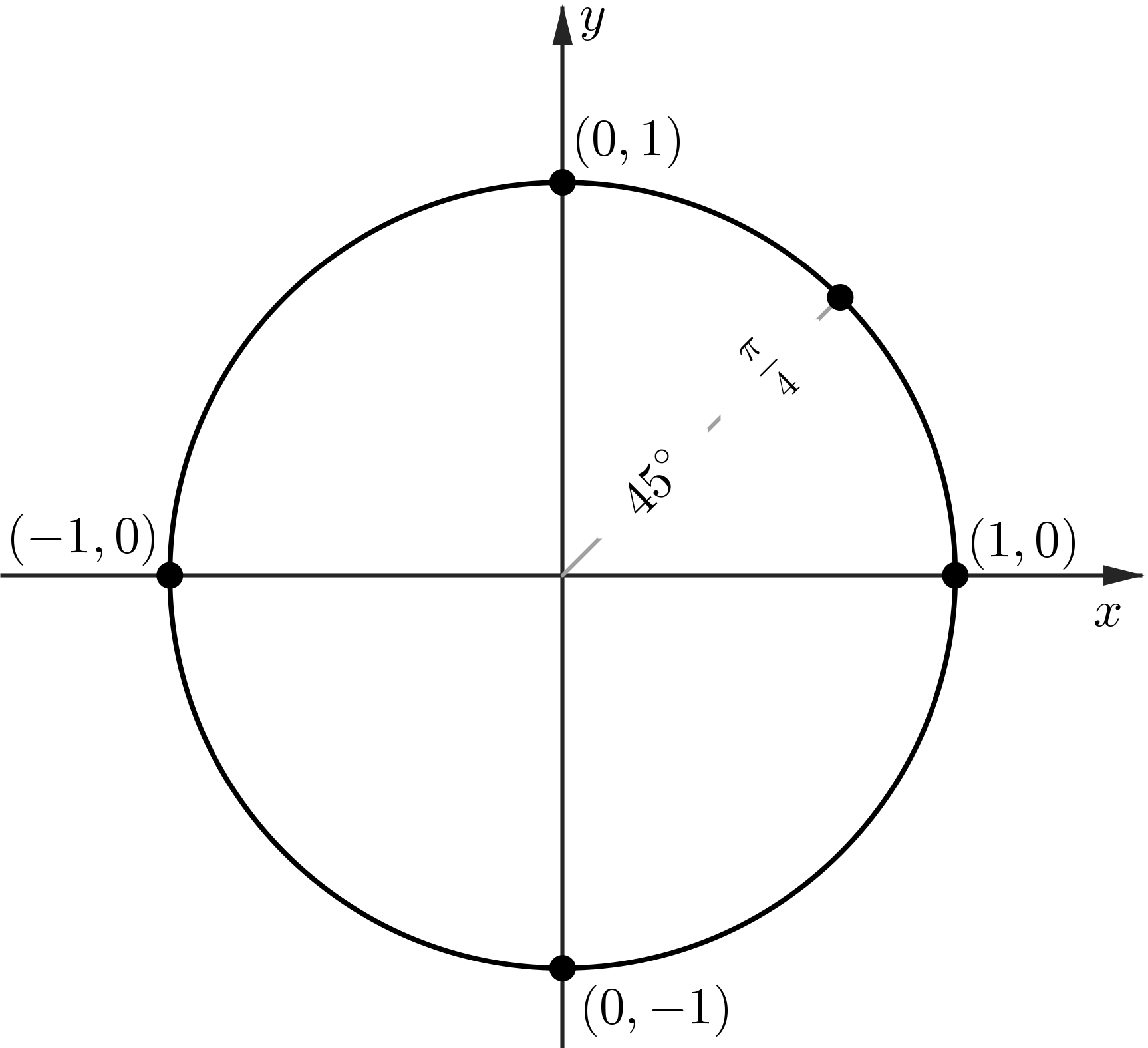
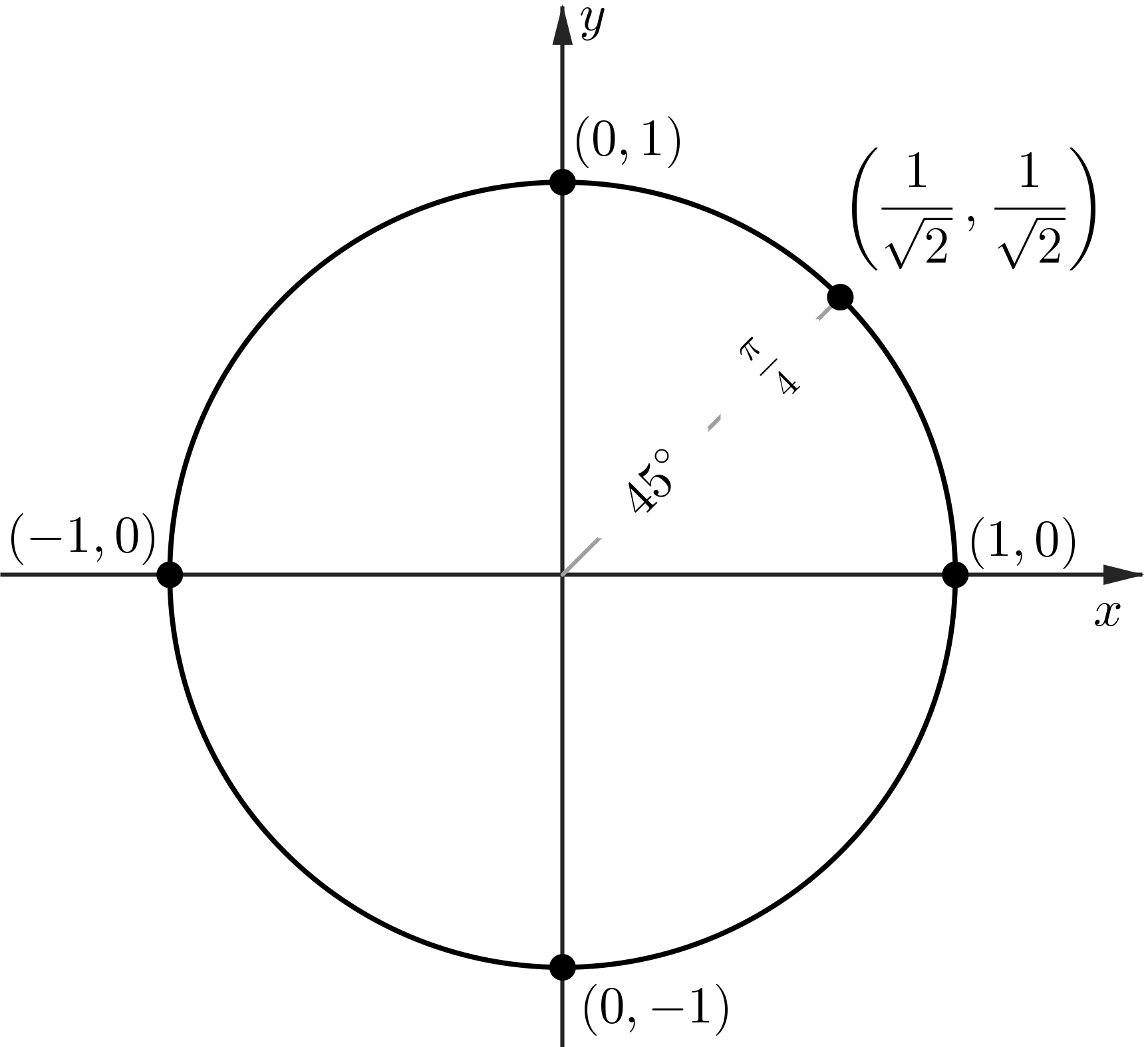
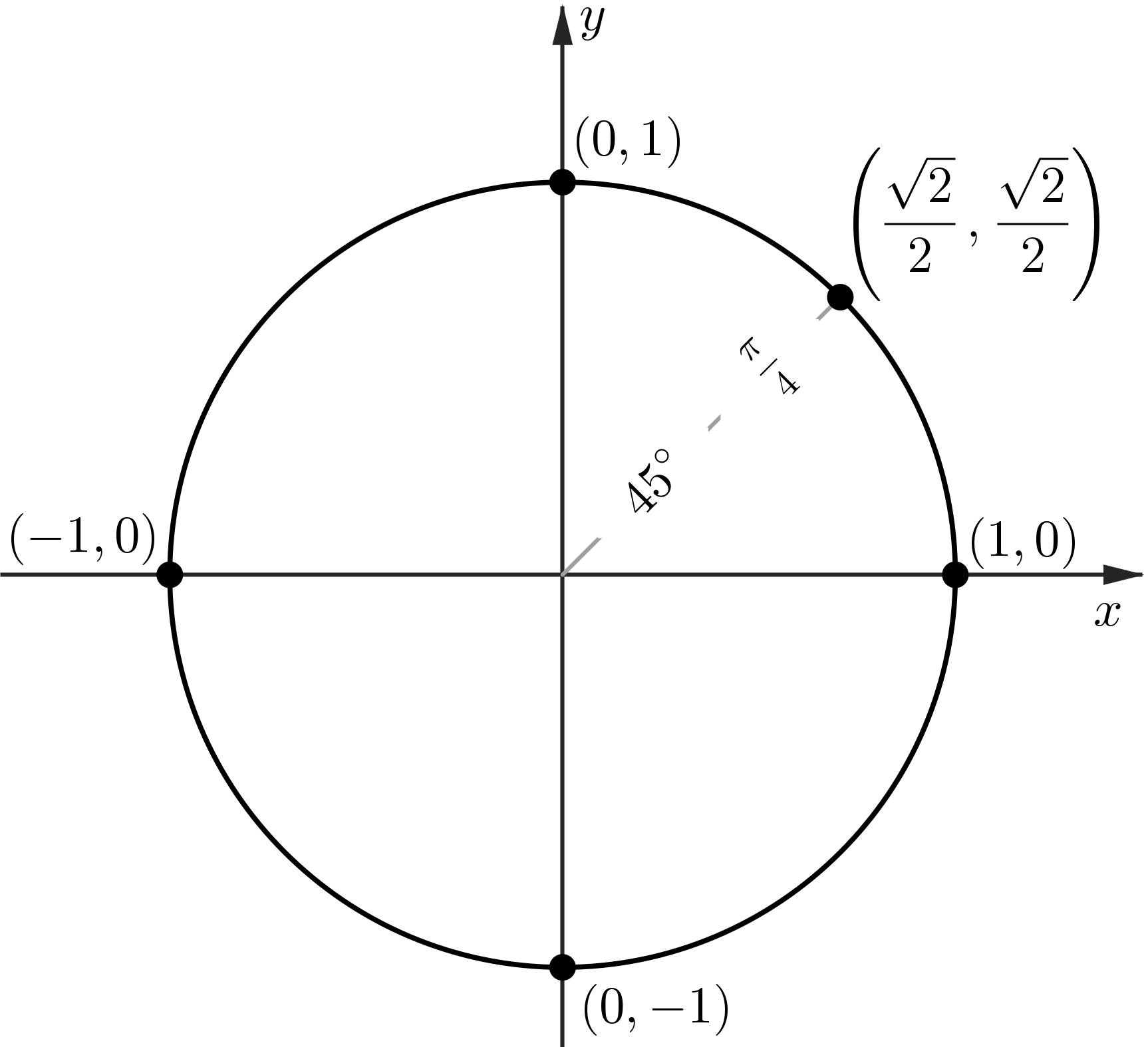
|
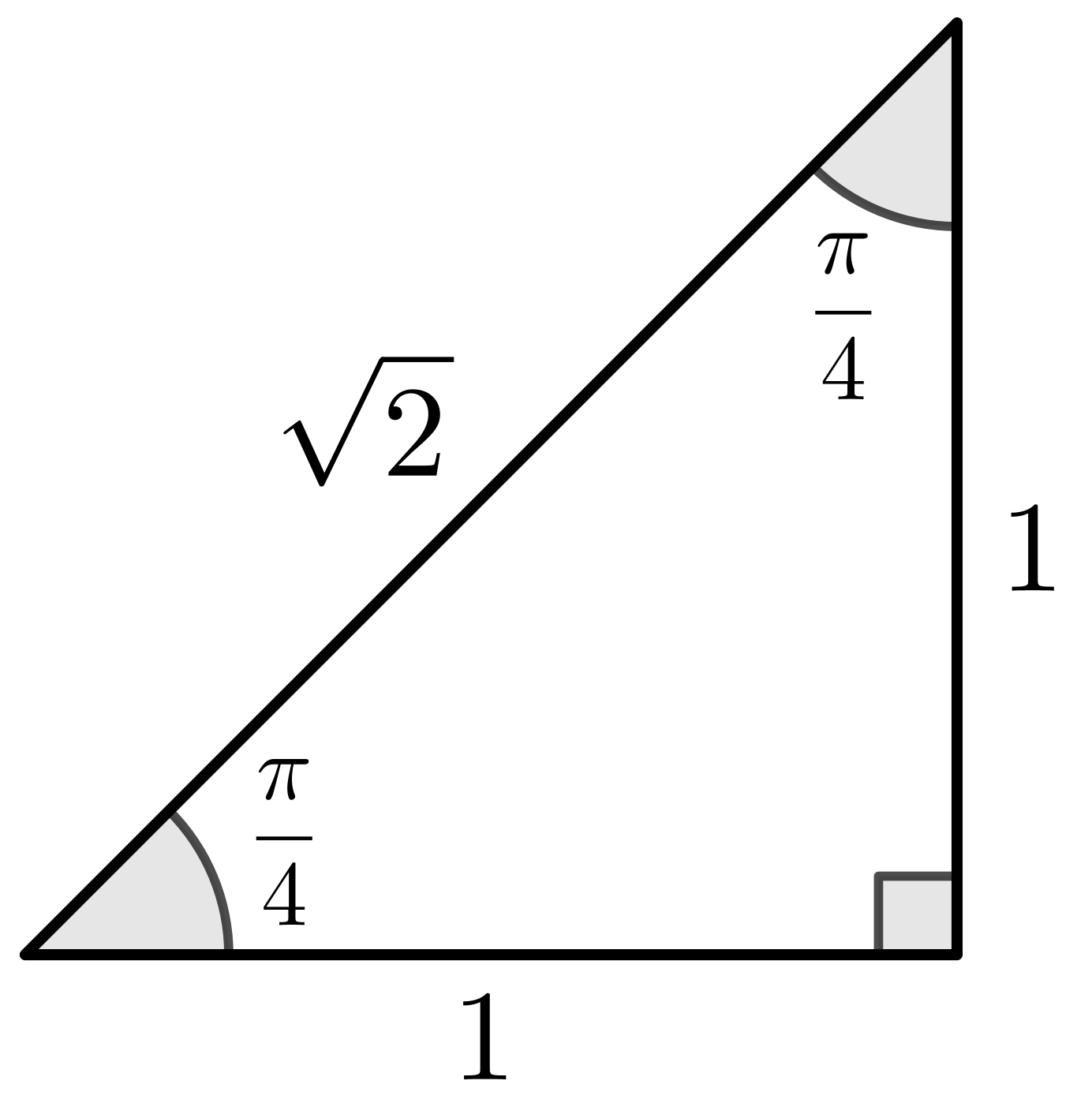
|
The Unit Circle: sin and cos at $60^\circ$ or $\pi/3$
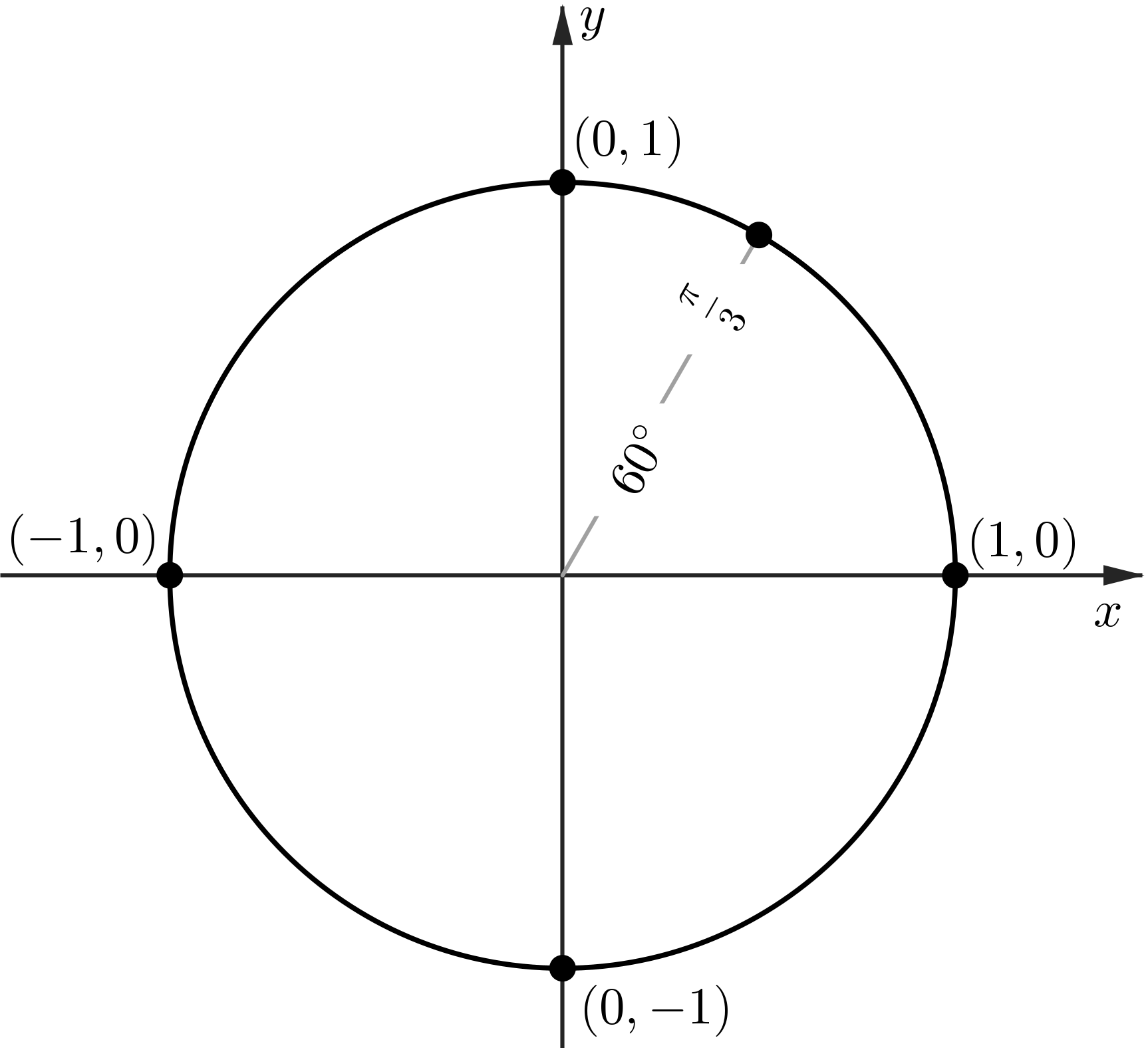
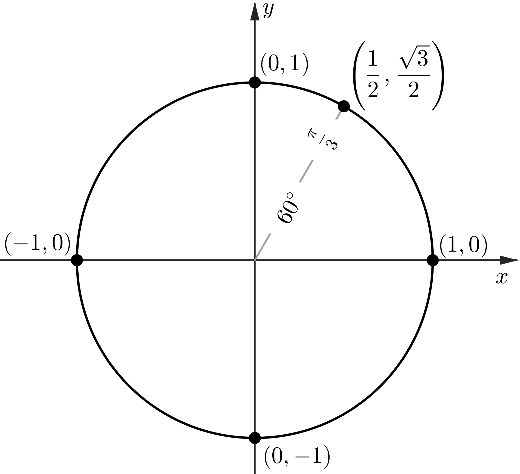
|
|
The Unit Circle
The Unit Circle
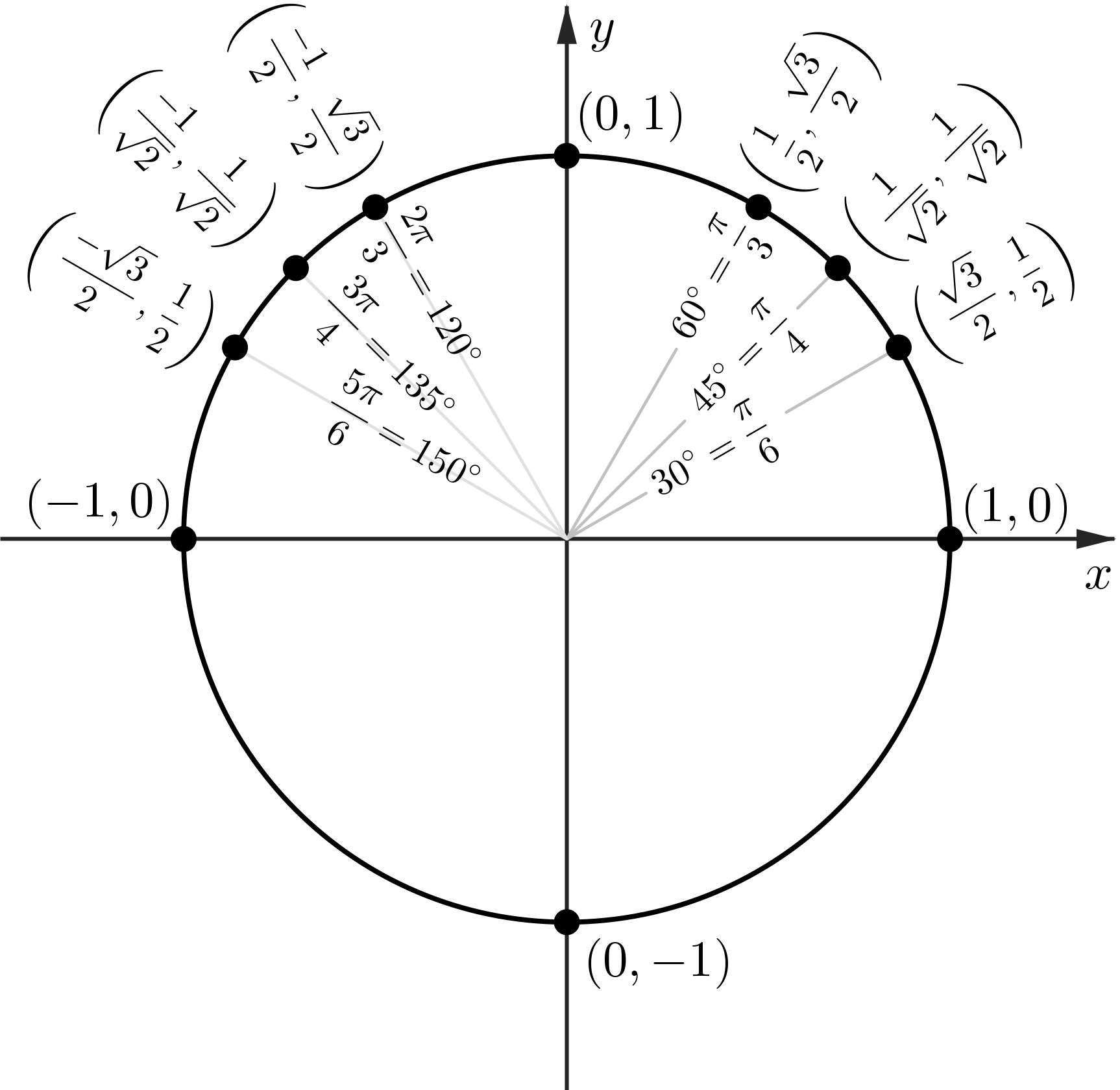
The Unit Circle
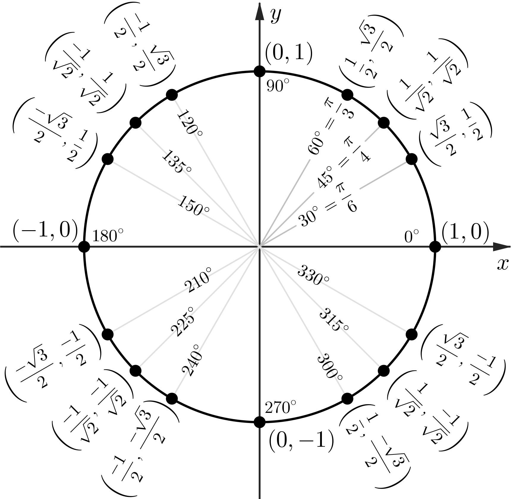
The Unit Circle
Graphing trigonometric functions (sin)

Graphing trigonometric functions (sin)

Graphing trigonometric functions (sin)

Graphing trigonometric functions (cos)

Graphing trigonometric functions (cos)
Graphing trigonometric functions (cos)

The unit circle and it's relationship with sin and cos
Graphing trigonometric functions (sin & cos in degrees)


Graphing trigonometric functions (sin & cos in radians)


The unit circle and Trigonometric functions
Summary of Elementary functions
* We won't use these functions in this course.
📝 Practice 😃
📝 Practice: Logarithms
Find without the calculator:
- \(\log(1000)\)
- \(\ln \left(e^3\right)\)
- \(10^{\log(3)}\)
- \(e^{\ln(4)}\)
- \(\log(25)+ \log(4)\)
📝 Practice: Exponential functions
The 🦠 bacteria population is described by the following equation:
\(P(t) = 500 \times 10 ^{0.2 t}\)
$t$ is measured in years.
- Write this as an exponent with base $e$.
- Is the population growing or shrinking?
- What will be the population of bacteria after 3 years?
- After how long does it double or halve? - pick one based on answers to part 2.
- When would it reach a population of 200? of 2,000? -pick one based on answers to part 1.
Solution part 1: Write with base e
\(P(t) = 500 \times 10 ^{0.2 t}\)
We rewrite:
\( 10^{0.2t} = \exp\left( \ln\left(10^{0.2 t} \right) \right) \) \( = \exp\big( 0.2 t\ln\left(10 \right) \big) \) \( = e^{0.2t \ln(10)} \)
So \(\; P(t) = 500\, e^{(0.2\ln 10)\, t} \)
Consider 4 decimal: \(\; 0.2\ln (10) \approx 0.4605\):
Then \(\; P(t) =500\, e^{0.4605 t} \)
Solution part 2: Growing or shrinking?
\(P(t) = 500 \times 10 ^{0.2 t}\)
The exponent coefficient is positive:
\(0.2 > 0\;\; \) \(\Rightarrow \;\; \) population grows.
So the bacteria population is growing.
Solution part 3: Population after 3 years
\(P(t) = 500 \times 10 ^{0.2 t}\)
Compute:
\( P(3) = 500 \times 10^{0.2 (3)} \) \( = 500 \times 10^{0.6} \)
\(10^{0.6} \approx 3.981\)
\[ P(3) \approx 500 \times 3.981 = 1990.5 \]
So after 3 years: \(\approx 1991\) bacteria
Solution part 4: Doubling time
Here we need to solve: $ 500 \times 10^{0.2t} = 1000 $
Divide both sides by 500:\(\; 10^{0.2t} = 2 \)
Take log base 10:
\[ 0.2t = \log_{10}(2) \]
\( \Ra \;t = \dfrac{\log_{10}(2)}{0.2} \) \(\approx \dfrac{0.3010}{0.2} \) \( = 1.505 \)
Doubling time ≈ 1.51 years
Solution part 5: When does it reach a chosen population?
Consider population = $2\,000.$ Solve: $500 \times 10^{0.2t} = 2\,000 $
Divide both sides by 500:\(\; 10^{0.2t} = 4 \)
Take log base 10: \(\;0.2t = \log_{10}(4) = 0.6021 \)
\[ t = \frac{0.6021}{0.2} = 3.01 \]
So the population reaches 2,000 after ≈ 3.0 years.
Exploring functions
The Normal Distribution

The Normal Distribution
$ \large f_X(x; \mu, \sigma) =\ds \frac{1}{\sigma \sqrt{2\pi}} e^{-\frac{1}{2} \left( \frac{x - \mu}{\sigma} \right)^2}, $
$x \in \R,\, \mu \in \R, \sigma > 0,$
The Normal Distribution
$ \large N\left(\mu, \sigma^2\right) =\ds \frac{1}{\sigma \sqrt{2\pi}} e^{-\frac{1}{2} \left( \frac{x - \mu}{\sigma} \right)^2}$
We write $X\sim N\left(\mu, \sigma^2\right)$:
$X$ is normally distributed with mean $\mu$ and variance $\sigma^2.$
The Normal Distribution
Areas under the Standard Normal Distribution
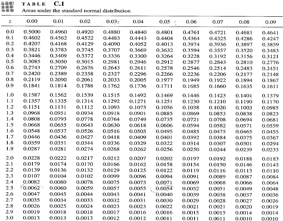
Areas under the Standard Normal Distribution
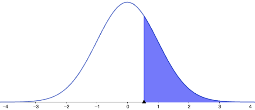
Now we use computers or calculators 👩💻!
See for example this one: |
|
Where functions are used?
🌡️ Temperature Conversion
Convert Celsius to Fahrenheit:
\[ F(C) = \frac{9}{5}C + 32 \]
- Linear function
- Slope: \( \dfrac{9}{5} \)
- Y-intercept: \( 32 \)
Used in weather reports, lab experiments, etc.
📊 Linear Regression
Predicting height from age: Suppose we collect data from children aged 2 to 13 and record their heights.


📊 Linear Regression
Predicting height from age:
The data points suggest a linear trend:
\[ h(a) = 6.58a + 70.36 \]
📈 Linear Regression
Predicting height from age:
The data points suggest a linear trend:
\[ h(a) = 6.58a + 70.36 \]
- \( a \): age in years
- \( h(a) \): predicted height in cm
- Slope \( 6.58 \): average growth per year
This line is the line of best fit — found using linear regression.
Polynomial Regression
$y = a_0 + a_1x + a_2x^2 + \cdots + a_nx^n + \epsilon$
We look for a least squares polynomial function of best fit.
🔬 Hooke's Law (Spring Force)
Force needed to stretch a spring:
\[ F(x) = -kx \]
- Linear function
- \( x \): displacement in meters
- \( k \): spring constant (stiffness)
Used in physics, biomechanics, engineering.
We consider the differential equation: \(\ds m \frac{d^2 x}{dt^2}+k x = 0.\)
🔬 Hooke's Law (Spring Force)
The undamped spring
Use mouse to drag mass and release.
$x(t) = A \sin \left(\omega t \right)$
🔬 Hooke's Law (Spring Force)
Damped spring. Use mouse to drag mass and release.
☕️ Law of Cooling & 🧫 Population Growth

|

|
| \(T(t)=\left(T_0-T_m\right) e^{-kt} + T_m\) | $\ds P(t) = \frac{\theta P_0 e^{rt}}{\theta-P_0+P_0e^{rt}}$ |
💊 Medicine in the Body
Drug concentration decreases over time:
\[ C(t) = C_0 e^{-kt} \]
- Exponential decay
- \( C_0 \): initial concentration
- \( k \): decay constant
Models how the body metabolizes medicine.
💊 Medicine in the Body
\[ C(t) = 100 e^{-0.3t} \]
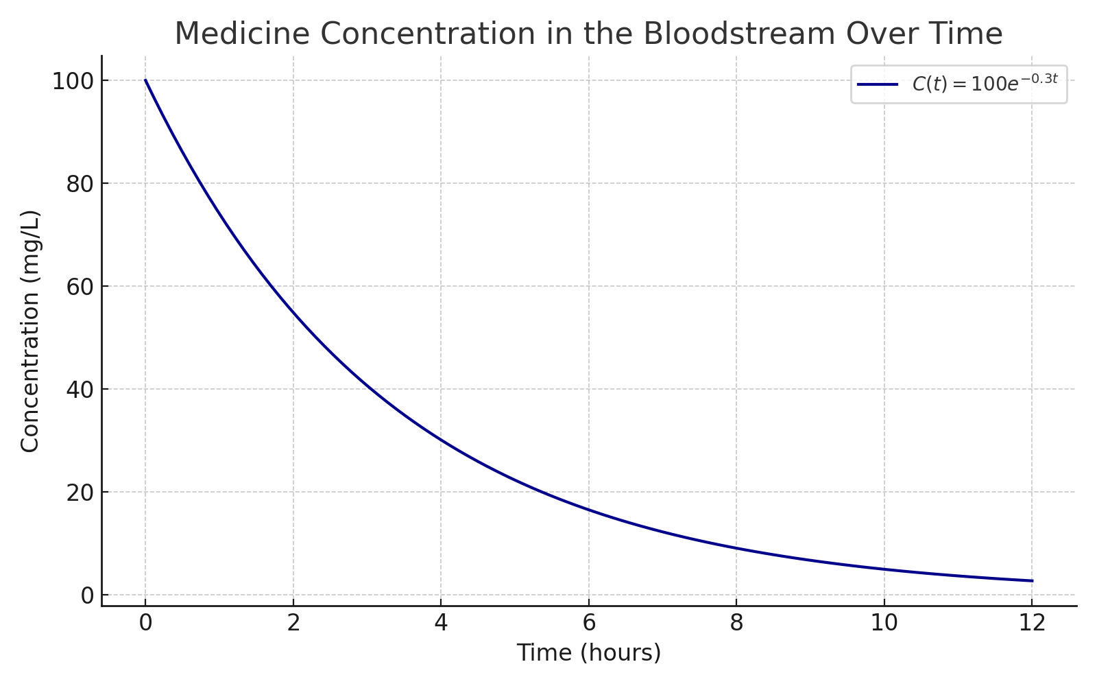
This is a classic example of exponential decay, useful in pharmacology for understanding how a drug's concentration diminishes after administration.
📚 Diminishing Returns in Learning
Modelling learning over time:
Early learning is fast, then progress slows:
\[L(t) = 20 \ln(t + 1)\]
- $t$: time spent learning (hours)
- $L(t)$: performance level
- Logarithmic growth: quick gains at first, then slower improvement
This model captures the idea of diminishing returns in real learning scenarios.
📚 Diminishing Returns in Learning
\[ L(t) = 20 \ln(t + 1) \]
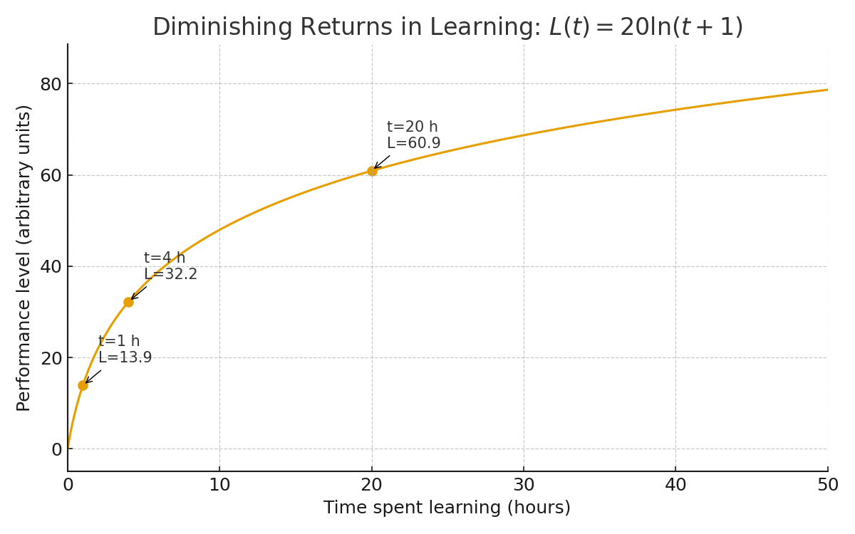
This model shows how learning improves quickly at first and then slows over time, a classic example of diminishing returns in skill acquisition.
Trigonometric functions: Procedural Landscape Generation
\[ f(\mathbf{x}) = \sum_{i=0}^{N-1} A_i \cdot \big[\cos\left(2\pi \, \mathbf{k}_i \cdot \mathbf{x} + \phi_i\right) + \sin\left(2\pi \, \mathbf{k}_i \cdot \mathbf{x} + \theta_i\right)\big] \]
Combined with Linear Algebra
to visualise the 3D surface! 🤯
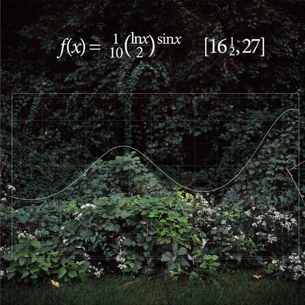
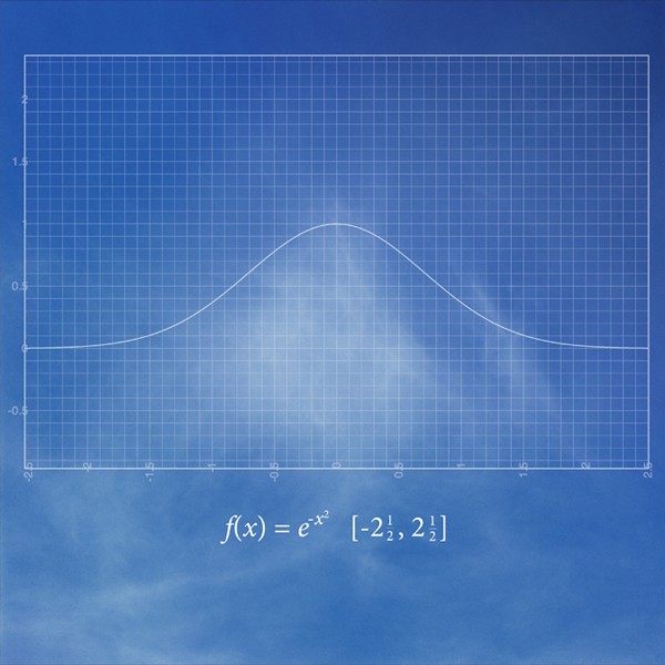
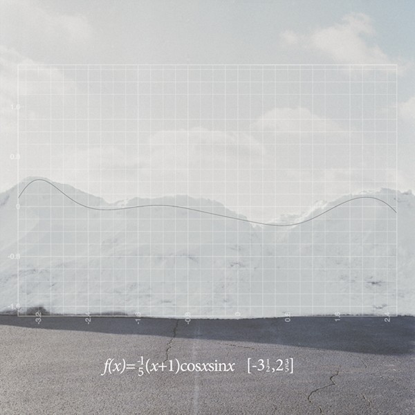
Computer Graphics & Art
|
|
$f(x) = \sqrt{6^2-x^2}$
$g(x) = 2 + 2 \sin(\text{floor}(x-t) 4321)$ $h_k(x) = \dfrac{-5}{k}+\dfrac{2}{5}, $ $\qquad k=0,1,\ldots, 10$ |
Art with functions in Excel

|
Try it yourself! 🌼😊 Tutorial: Painting with Maths in Google Sheets by Iñigo Quilez |
Computer Graphics & Art
|
$R =13 + 3\left(\dfrac{1}{2} + \dfrac{1}{2} \sin \left(2\pi t + \dfrac{z}{3}\right)\right)^4$ $y = z -\abs{x}\sqrt{ \dfrac{20 - \abs{x}}{35} }$ $x^{2}+y^{2}+z^{2}=R$ |
Computer Graphics & Art
\( \ds \sum_{k} w_k \left|\sin\!\left(\text{space}+\text{time}+\text{frequency}_k\right)\right| \)
Found Functions
Time in a Bottle by Jim Croce
That's all for today!
See you in Week 6!