1015SCG - Lecture 11

Quantitative Reasoning

1015SCG

Lecture 11

A brief intro to `R`

What is `R`?

R is a programming language for:

Statistical computing
Data analysis
Data visualisation

It is widely used in:

Statistics
Data science
Scientific research
Education

R is open-source
and free! 😀

rdrr.io

Basic `R` Syntax

Code	Output
`# Assign values using <- x <- 5 y <- 2`
`# Basic arithmetic x + y x * y x / y`	`> 7` `> 10` `> 2.5`
`# Create a vector v <- c(1, 2, 3, 4, 5) mean(v)`	`> 3`

`R` studio

`R` in Visual Studio Code

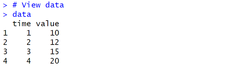
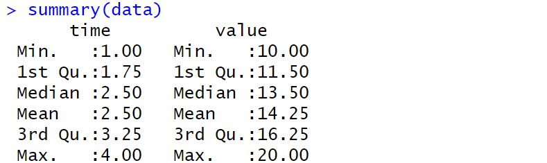
Working with Data

Code Output

Code	Output
`# Create a data frame data <- data.frame( time = c(1, 2, 3, 4), value = c(10, 12, 15, 20) )` `# View data data summary(data)` `# Simple plot plot(data$time, data$value)`


# Create a data frame
data <- data.frame(
  time = c(1, 2, 3, 4),
  value = c(10, 12, 15, 20)
)


# View data
data
summary(data)


# Simple plot
plot(data$time, data$value)

📖 Documentation

`R` code

Include data manually

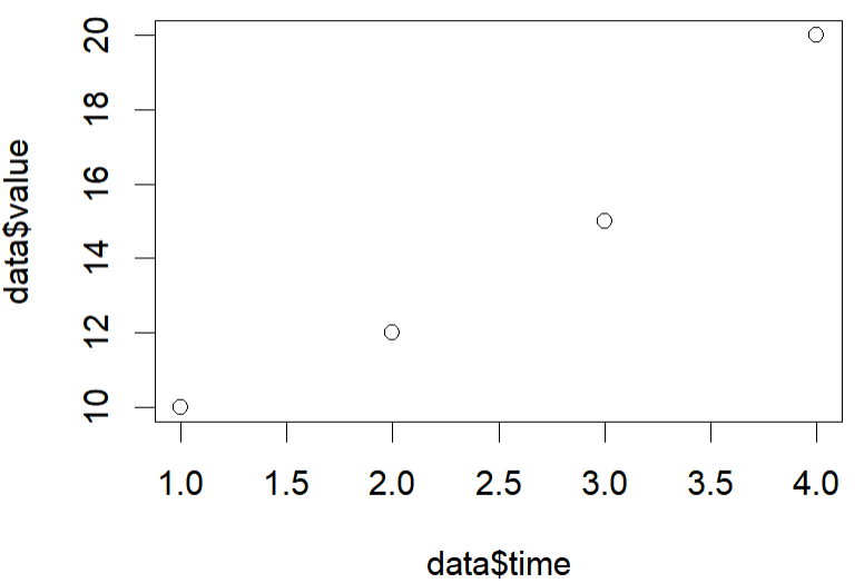
Scatter plot

						# -------------------------
# Data (entered directly)
# -------------------------
# Time variable
t <- c(
  0.246, 0.492, 0.738, 0.984, 1.23, 1.476, 1.722, 1.968, 2.214, 2.46,
  2.706, 2.952, 3.198, 3.444, 3.69, 3.936, 4.182, 4.428, 4.674, 4.92,
  5.166, 5.412, 5.658, 5.904, 6.15, 6.396, 6.642, 6.888, 7.134, 7.38,
  7.626, 7.872, 8.118, 8.364, 8.61, 8.856, 9.102, 9.348, 9.594, 9.84
)
# Activity variable
y <- c(
  908.3475159, 788.1263257, 668.9006718, 554.6124143, 521.6023327,
  392.2851028, 406.7494851, 323.1341532, 282.4183865, 236.0078351,
  200.7706532, 199.8517187, 169.289558, 148.5259409, 127.8568286,
  98.33976068, 87.93068585, 87.27796212, 73.97245838, 66.69058729,
  56.82525099, 50.73912403, 39.4075143, 34.33557193, 32.61742786,
  25.96560655, 22.36805436, 19.64146032, 16.71665582, 14.63554653,
  12.49930957, 12.4940735, 9.520718439, 8.135601522, 7.562147198,
  6.250336563, 5.376122231, 4.91574392, 4.449048126, 3.892785478
)

# -------------------------
# Scatter plot
# -------------------------
plot(time, activity,
     pch = 19,                        # Solid circular plotting symbol
     cex = 1.5,                       # Size of the plotting points
     col = rgb(0, 0, 0.7, 0.7),       # Blue colour with transparency
     xlab = "time [sec]",             # Label for the x-axis
     ylab = "activity [decays/sec]",  # Label for the y-axis
     main = "Radioactive decay data", # Title of the plot
     las = 1)                         # Axis labels drawn horizontally

grid()                                # Add a background grid to the plot

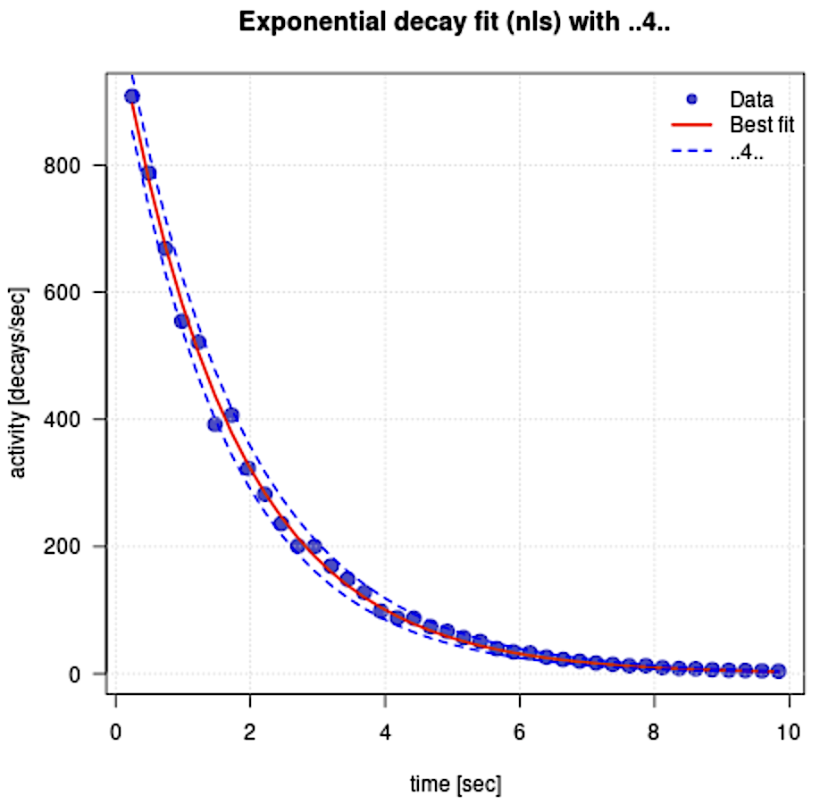
Scatter plot & Trending line

						# -------------------------
# Data (entered directly)
# -------------------------
# Time variable
t <- c(
  0.246, 0.492, 0.738, 0.984, 1.23, 1.476, 1.722, 1.968, 2.214, 2.46,
  2.706, 2.952, 3.198, 3.444, 3.69, 3.936, 4.182, 4.428, 4.674, 4.92,
  5.166, 5.412, 5.658, 5.904, 6.15, 6.396, 6.642, 6.888, 7.134, 7.38,
  7.626, 7.872, 8.118, 8.364, 8.61, 8.856, 9.102, 9.348, 9.594, 9.84
)
# Activity variable
y <- c(
  908.3475159, 788.1263257, 668.9006718, 554.6124143, 521.6023327,
  392.2851028, 406.7494851, 323.1341532, 282.4183865, 236.0078351,
  200.7706532, 199.8517187, 169.289558, 148.5259409, 127.8568286,
  98.33976068, 87.93068585, 87.27796212, 73.97245838, 66.69058729,
  56.82525099, 50.73912403, 39.4075143, 34.33557193, 32.61742786,
  25.96560655, 22.36805436, 19.64146032, 16.71665582, 14.63554653,
  12.49930957, 12.4940735, 9.520718439, 8.135601522, 7.562147198,
  6.250336563, 5.376122231, 4.91574392, 4.449048126, 3.892785478
)

# Provide reasonable starting values for the parameters
start_vals <- list(
  A = max(y),    # initial activity (approximate)
  k = -0.5       # decay constant (negative for decay)
)

# Fit exponential decay model y = A * exp(kx)
nls_fit <- nls(y ~ A * exp(k * x), start = start_vals)

# Extract fitted parameters
coef_fit <- coef(nls_fit)
A <- coef_fit["A"]
k <- coef_fit["k"]

# Confidence intervals for parameters
conf <- confint(nls_fit)

# Approximate standard errors (1σ) from 95% confidence intervals
A_err <- (conf["A", 2] - conf["A", 1]) / 4
k_err <- (conf["k", 2] - conf["k", 1]) / 4


# -------------------------
# Fitted curves
# -------------------------
# Best-fit curve
y_fit <- A * exp(k * x)
# ±4σ uncertainty envelopes
y_fit_upper <- (A + 4 * A_err) * exp((k + 4 * k_err) * x)
y_fit_lower <- (A - 4 * A_err) * exp((k - 4 * k_err) * x)


# -------------------------
# Plot
# -------------------------
plot(x, y,
     pch = 19,
     cex = 1.5,
     col = rgb(0, 0, 0.7, 0.7),
     xlab = "time [sec]",
     ylab = "activity [decays/sec]",
     main = "Exponential decay fit (nls) with ±4σ",
     las = 1)

grid()

lines(x, y_fit, col = "red", lwd = 2)
lines(x, y_fit_upper, col = "blue", lty = 2, lwd = 1.5)
lines(x, y_fit_lower, col = "blue", lty = 2, lwd = 1.5)

legend("topright",
       legend = c("Data", "Best fit", "±4σ"),
       col = c(rgb(0,0,0.7,0.7), "red", "blue"),
       pch = c(19, NA, NA),
       lty = c(NA, 1, 2),
       lwd = c(NA, 2, 1.5),
       bty = "n")


# -------------------------
# Output results
# -------------------------
cat("Exponential model (nls):\n")
cat(sprintf("A(t) = %.3f * exp(%.4f * t)\n", A, k))
cat(sprintf("Estimated ±1σ: A = %.3f ± %.3f, k = %.4f ± %.4f\n",
            A, A_err, k, k_err))

# Value of the fitted model at t = 0
t0 <- 0
A0 <- A * exp(k * t0)
cat(sprintf("A(0) = %.3f\n", A0))

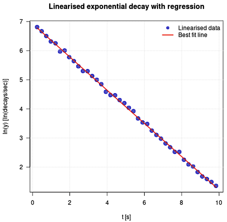
Linearisation

						# -------------------------
# Data (entered directly)
# -------------------------
t <- c(
  0.246, 0.492, 0.738, 0.984, 1.23, 1.476, 1.722, 1.968, 2.214, 2.46,
  2.706, 2.952, 3.198, 3.444, 3.69, 3.936, 4.182, 4.428, 4.674, 4.92,
  5.166, 5.412, 5.658, 5.904, 6.15, 6.396, 6.642, 6.888, 7.134, 7.38,
  7.626, 7.872, 8.118, 8.364, 8.61, 8.856, 9.102, 9.348, 9.594, 9.84
)

y <- c(
  908.3475159, 788.1263257, 668.9006718, 554.6124143, 521.6023327,
  392.2851028, 406.7494851, 323.1341532, 282.4183865, 236.0078351,
  200.7706532, 199.8517187, 169.289558, 148.5259409, 127.8568286,
  98.33976068, 87.93068585, 87.27796212, 73.97245838, 66.69058729,
  56.82525099, 50.73912403, 39.4075143, 34.33557193, 32.61742786,
  25.96560655, 22.36805436, 19.64146032, 16.71665582, 14.63554653,
  12.49930957, 12.4940735, 9.520718439, 8.135601522, 7.562147198,
  6.250336563, 5.376122231, 4.91574392, 4.449048126, 3.892785478
)

# -------------------------
# Linearisation: ln(y) = ln(A) + k*t
# -------------------------
lny <- log(y)
lin_fit <- lm(lny ~ t)

# Regression parameters
k <- coef(lin_fit)[2]
lnA <- coef(lin_fit)[1]
A <- exp(lnA)

# Standard errors
se <- summary(lin_fit)$coefficients[, "Std. Error"]
k_err <- se[2]
lnA_err <- se[1]
A_err <- A * lnA_err  # propagated error

# R-squared
r_squared <- summary(lin_fit)$r.squared

# Fitted line
lny_fit <- lnA + k * t
y_fit <- A * exp(k * t)

# -------------------------
# Standard error of regression
# -------------------------
n <- length(t)
residuals <- lny - lny_fit
s <- sqrt(sum(residuals^2) / (n - 2))
t_mean <- mean(t)
Sxx <- sum((t - t_mean)^2)
k_err_alt <- s / sqrt(Sxx)
lnA_err_alt <- s * sqrt(1/n + t_mean^2 / Sxx)

# -------------------------
# Plot
# -------------------------
plot(t, lny,
     pch = 19, cex = 1.5, col = rgb(0,0,0.7,0.7),
     xlab = "t [s]",
     ylab = "ln(y) [ln(decays/sec)]",
     main = "Linearised exponential decay with regression",
     las = 1)
grid()
lines(t, lny_fit, col = "red", lwd = 2)
legend("topright",
       legend = c("Linearised data", "Best fit line"),
       col = c(rgb(0,0,0.7,0.7), "red"),
       pch = c(19, NA),
       lty = c(NA, 1),
       lwd = c(NA, 2),
       bty = "n")

# -------------------------
# Half-life computation
# -------------------------
t_half <- log(2) / -k
t_half_err <- log(2) / k^2 * k_err

# -------------------------
# Prediction at t = 5.535 s
# -------------------------
t_pred <- 5.535
sigma_A <- A * lnA_err
sigma_y <- sqrt( (exp(k*t_pred) * sigma_A)^2 + (A * t_pred * exp(k*t_pred) * k_err)^2 )
y_pred <- A * exp(k * t_pred)

# -------------------------
# Output results
# -------------------------
cat("-----------------------\n")
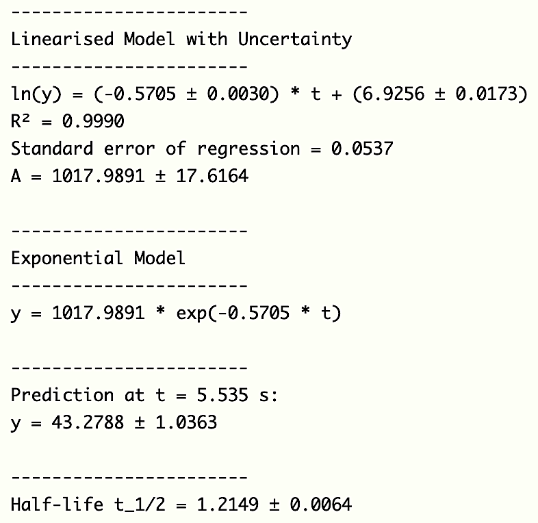
cat("Linearised Model with Uncertainty\n")
cat("-----------------------\n")
cat(sprintf("ln(y) = (%.4f ± %.4f) * t + (%.4f ± %.4f)\n", k, k_err, lnA, lnA_err))
cat(sprintf("R² = %.4f\n", r_squared))
cat(sprintf("Standard error of regression = %.4f\n", s))
cat(sprintf("A = %.4f ± %.4f\n\n", A, A_err))

cat("-----------------------\n")
cat("Exponential Model\n")
cat("-----------------------\n")
cat(sprintf("y = %.4f * exp(%.4f * t)\n\n", A, k))

cat("-----------------------\n")
cat(sprintf("Prediction at t = %.3f s:\n", t_pred))
cat(sprintf("y = %.4f ± %.4f\n\n", y_pred, sigma_y))

cat("-----------------------\n")
cat(sprintf("Half-life t_1/2 = %.4f ± %.4f\n", t_half, t_half_err))

One Sample Student t-test

						# -------------------------
# Data
# -------------------------
data <- c(275.0266497, 255.0311768, 293.8473708, 267.1938408, 242.3487616)
mu0 <- 246.966  # hypothesised mean

# -------------------------
# One-sample t-test
# -------------------------
t_test <- t.test(data, mu = mu0)

# Extract t-statistic
t_stat <- t_test$statistic

# Degrees of freedom
df <- t_test$parameter

# Two-tailed t-critical value (alpha = 0.02)
alpha <- 0.02
t_critical <- qt(1 - alpha/2, df)

# -------------------------
# Output results
# -------------------------
cat("t-statistic:", t_stat, "\n")
cat("t-critical (two-tailed, alpha = 0.02):", t_critical, "\n")\

`R` code

Load data from local folder

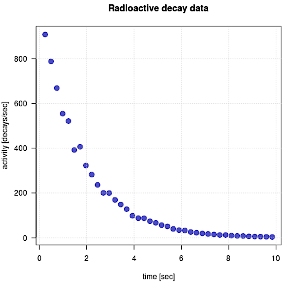
Scatter plot

						# -------------------------
# Load data
# -------------------------
getwd()          # Display the current working directory
list.files()     # List all files in the current working directory

# Set the working directory to the folder containing decay3.csv
setwd("C:/Users/YourUserName/Folder/R-code")

# Read the CSV file into a data frame
data <- read.csv("decay3.csv")

# Show the data in the csv file
View(data)

# Extract the first column (time values)
time <- data[[1]]

# Extract the second column (activity values)
activity <- data[[2]]

# -------------------------
# Scatter plot
# -------------------------

plot(time, activity,
     pch = 19,                        # Solid circular plotting symbol
     cex = 1.5,                       # Size of the plotting points
     col = rgb(0, 0, 0.7, 0.7),       # Blue colour with transparency
     xlab = "time [sec]",             # Label for the x-axis
     ylab = "activity [decays/sec]",  # Label for the y-axis
     main = "Radioactive decay data", # Title of the plot
     las = 1)                         # Axis labels drawn horizontally

grid()                                # Add a background grid to the plot

Scatter plot & Trending line

						# -------------------------
# Load data
# -------------------------
getwd()          # Show current working directory (diagnostic)
list.files()     # Show files in the current working directory

# Set working directory to where decay3.csv is stored
setwd("C:/Users/YourUserName/Folder/R-code")

# Read the CSV file into a data frame
data <- read.csv("decay3.csv")

# Assign columns to variables used in the model
x <- data[[1]]   # time values
y <- data[[2]]   # activity values


# -------------------------
# Non-linear fit using nls
# -------------------------
# Provide reasonable starting values for the parameters
start_vals <- list(
  A = max(y),    # initial activity (approximate)
  k = -0.5       # decay constant (negative for decay)
)
# Fit exponential decay model y = A * exp(kx)
nls_fit <- nls(y ~ A * exp(k * x), start = start_vals)
# Extract fitted parameters
coef_fit <- coef(nls_fit)
A <- coef_fit["A"]
k <- coef_fit["k"]
# Confidence intervals for parameters
conf <- confint(nls_fit)
# Approximate standard errors (1σ) from 95% confidence intervals
A_err <- (conf["A", 2] - conf["A", 1]) / 4
k_err <- (conf["k", 2] - conf["k", 1]) / 4


# -------------------------
# Fitted curves
# -------------------------
# Best-fit curve
y_fit <- A * exp(k * x)
# ±4σ uncertainty envelopes
y_fit_upper <- (A + 4 * A_err) * exp((k + 4 * k_err) * x)
y_fit_lower <- (A - 4 * A_err) * exp((k - 4 * k_err) * x)


# -------------------------
# Plot
# -------------------------
plot(x, y,
     pch = 19,
     cex = 1.5,
     col = rgb(0, 0, 0.7, 0.7),
     xlab = "time [sec]",
     ylab = "activity [decays/sec]",
     main = "Exponential decay fit (nls) with ±4σ",
     las = 1)

grid()

lines(x, y_fit, col = "red", lwd = 2)
lines(x, y_fit_upper, col = "blue", lty = 2, lwd = 1.5)
lines(x, y_fit_lower, col = "blue", lty = 2, lwd = 1.5)

legend("topright",
       legend = c("Data", "Best fit", "±4σ"),
       col = c(rgb(0,0,0.7,0.7), "red", "blue"),
       pch = c(19, NA, NA),
       lty = c(NA, 1, 2),
       lwd = c(NA, 2, 1.5),
       bty = "n")


# -------------------------
# Output results
# -------------------------
cat("Exponential model (nls):\n")
cat(sprintf("A(t) = %.3f * exp(%.4f * t)\n", A, k))
cat(sprintf("Estimated ±1σ: A = %.3f ± %.3f, k = %.4f ± %.4f\n",
            A, A_err, k, k_err))

# Value of the fitted model at t = 0
t0 <- 0
A0 <- A * exp(k * t0)
cat(sprintf("A(0) = %.3f\n", A0))

Linearisation

						# -------------------------
# Load data
# -------------------------
getwd()          # Display current working directory (diagnostic)
list.files()     # List files in the current working directory

# Set working directory to the folder containing decay3.csv
setwd("C:/Users/YourUserName/Folder/R-code")

# Read the CSV file into a data frame
data <- read.csv("decay3.csv", header = TRUE)

# -------------------------
# Extract columns safely
# -------------------------
# If the CSV file has column names "time" and "activity",
# use them; otherwise, assume the first two columns

if (!("time" %in% colnames(data)) | !("activity" %in% colnames(data))) {
  time <- data[, 1]      # first column: time
  activity <- data[, 2]  # second column: activity
} else {
  time <- data$time
  activity <- data$activity
}

# -------------------------
# Linearisation: ln(y) = ln(A) + k t
# -------------------------
# Take the natural logarithm of the activity data
lny <- log(activity)

# Perform linear regression on the linearised model
lin_fit <- lm(lny ~ time)

# -------------------------
# Extract regression parameters
# -------------------------
k   <- coef(lin_fit)[2]   # slope (decay constant)
lnA <- coef(lin_fit)[1]   # intercept
A   <- exp(lnA)           # recover A from ln(A)

# -------------------------
# Parameter uncertainties
# -------------------------
# Standard errors from regression output
se <- summary(lin_fit)$coefficients[, "Std. Error"]

k_err   <- se[2]          # uncertainty in k
lnA_err <- se[1]          # uncertainty in ln(A)

# Propagate uncertainty from ln(A) to A
A_err <- A * lnA_err

# -------------------------
# Goodness of fit
# -------------------------
r_squared <- summary(lin_fit)$r.squared

# -------------------------
# Fitted models
# -------------------------
# Linearised fitted line
lny_fit <- lnA + k * time

# Corresponding exponential model
y_fit <- A * exp(k * time)

# -------------------------
# Standard error of regression
# -------------------------
n <- length(time)                 # number of data points
residuals <- lny - lny_fit        # residuals of linearised fit

# Standard error of the regression
s <- sqrt(sum(residuals^2) / (n - 2))

# Alternative expressions for parameter uncertainties
t_mean <- mean(time)
Sxx <- sum((time - t_mean)^2)

k_err_alt   <- s / sqrt(Sxx)
lnA_err_alt <- s * sqrt(1 / n + t_mean^2 / Sxx)

# -------------------------
# Plot (force refresh)
# -------------------------
graphics.off()   # Close any existing graphics device

plot(time, lny,
     pch = 19,
     cex = 1.5,
     col = rgb(0, 0, 0.7, 0.7),
     xlab = "t [s]",
     ylab = "ln(y) [ln(decays/sec)]",
     main = "Linearised exponential decay with regression",
     las = 1)

grid()
lines(time, lny_fit, col = "red", lwd = 2)

legend("topright",
       legend = c("Linearised data", "Best fit line"),
       col = c(rgb(0,0,0.7,0.7), "red"),
       pch = c(19, NA),
       lty = c(NA, 1),
       lwd = c(NA, 2),
       bty = "n")

# -------------------------
# Half-life computation
# -------------------------
# Half-life for exponential decay: t_1/2 = ln(2)/|k|
t_half <- log(2) / -k

# Uncertainty in half-life (propagation)
t_half_err <- log(2) / k^2 * k_err

# -------------------------
# Prediction at a specific time
# -------------------------
t_pred <- 5.535

# Propagate uncertainty in A and k
sigma_A <- A * lnA_err
sigma_y <- sqrt(
  (exp(k * t_pred) * sigma_A)^2 +
    (A * t_pred * exp(k * t_pred) * k_err)^2
)

# Predicted activity
y_pred <- A * exp(k * t_pred)

# -------------------------
# Output results
# -------------------------
cat("-----------------------\n")
cat("Linearised Model with Uncertainty\n")
cat("-----------------------\n")
cat(sprintf("ln(y) = (%.4f ± %.4f) t + (%.4f ± %.4f)\n",
            k, k_err, lnA, lnA_err))
cat(sprintf("R² = %.4f\n", r_squared))
cat(sprintf("Standard error of regression = %.4f\n", s))
cat(sprintf("A = %.4f ± %.4f\n\n", A, A_err))

cat("-----------------------\n")
cat("Exponential Model\n")
cat("-----------------------\n")
cat(sprintf("y = %.4f * exp(%.4f t)\n\n", A, k))

cat("-----------------------\n")
cat(sprintf("Prediction at t = %.3f s:\n", t_pred))
cat(sprintf("y = %.4f ± %.4f\n\n", y_pred, sigma_y))

cat("-----------------------\n")
cat(sprintf("Half-life t_1/2 = %.4f ± %.4f\n", t_half, t_half_err))

One Sample Student t-test

						# -------------------------
# Data
# -------------------------
# Sample data (observed measurements)
data <- c(275.0266497, 255.0311768, 293.8473708, 267.1938408, 242.3487616)

# Hypothesised population mean under H0
mu0 <- 246.966

# -------------------------
# One-sample t-test
# -------------------------

# Perform a one-sample Student t-test:
# H0: true mean = mu0
# H1: true mean ≠ mu0 (two-tailed by default)
t_test <- t.test(data, mu = mu0)

# Extract the t-statistic from the test result
t_stat <- t_test$statistic

# Degrees of freedom (n − 1 for one-sample t-test)
df <- t_test$parameter

# -------------------------
# Critical value
# -------------------------

# Significance level (alpha = 0.02 corresponds to a 98% confidence level)
alpha <- 0.02

# Two-tailed critical t-value:
# used for rejection region |t| > t_critical
t_critical <- qt(1 - alpha / 2, df)

# -------------------------
# Output results
# -------------------------

cat("t-statistic:", t_stat, "\n")
cat("t-critical (two-tailed, alpha = 0.02):", t_critical, "\n")

`Python` code

Include data manually

Scatter plot

						import numpy as np
import matplotlib.pyplot as plt
from scipy import stats

# -------------------------
# Data (entered directly)
# -------------------------
time = np.array([
    0.246, 0.492, 0.738, 0.984, 1.23, 1.476, 1.722, 1.968, 2.214, 2.46,
    2.706, 2.952, 3.198, 3.444, 3.69, 3.936, 4.182, 4.428, 4.674, 4.92,
    5.166, 5.412, 5.658, 5.904, 6.15, 6.396, 6.642, 6.888, 7.134, 7.38,
    7.626, 7.872, 8.118, 8.364, 8.61, 8.856, 9.102, 9.348, 9.594, 9.84
])

activity = np.array([
    908.3475159, 788.1263257, 668.9006718, 554.6124143, 521.6023327,
    392.2851028, 406.7494851, 323.1341532, 282.4183865, 236.0078351,
    200.7706532, 199.8517187, 169.289558, 148.5259409, 127.8568286,
    98.33976068, 87.93068585, 87.27796212, 73.97245838, 66.69058729,
    56.82525099, 50.73912403, 39.4075143, 34.33557193, 32.61742786,
    25.96560655, 22.36805436, 19.64146032, 16.71665582, 14.63554653,
    12.49930957, 12.4940735, 9.520718439, 8.135601522, 7.562147198,
    6.250336563, 5.376122231, 4.91574392, 4.449048126, 3.892785478
])

# -------------------------
# Scatter plot
# -------------------------
plt.figure(figsize=(6, 4))
plt.scatter(time, activity, s=40, alpha=0.7)

plt.xlabel("time [sec]")
plt.ylabel("activity [decays/sec]")
plt.title("Radioactive decay data")
plt.grid(True)
plt.show()

Scatter plot & Trending line

						import numpy as np
import matplotlib.pyplot as plt
from scipy import stats

# -------------------------
# Data (entered directly)
# -------------------------
x = np.array([
    0.246, 0.492, 0.738, 0.984, 1.23, 1.476, 1.722, 1.968, 2.214, 2.46,
    2.706, 2.952, 3.198, 3.444, 3.69, 3.936, 4.182, 4.428, 4.674, 4.92,
    5.166, 5.412, 5.658, 5.904, 6.15, 6.396, 6.642, 6.888, 7.134, 7.38,
    7.626, 7.872, 8.118, 8.364, 8.61, 8.856, 9.102, 9.348, 9.594, 9.84
])

y = np.array([
    908.3475159, 788.1263257, 668.9006718, 554.6124143, 521.6023327,
    392.2851028, 406.7494851, 323.1341532, 282.4183865, 236.0078351,
    200.7706532, 199.8517187, 169.289558, 148.5259409, 127.8568286,
    98.33976068, 87.93068585, 87.27796212, 73.97245838, 66.69058729,
    56.82525099, 50.73912403, 39.4075143, 34.33557193, 32.61742786,
    25.96560655, 22.36805436, 19.64146032, 16.71665582, 14.63554653,
    12.49930957, 12.4940735, 9.520718439, 8.135601522, 7.562147198,
    6.250336563, 5.376122231, 4.91574392, 4.449048126, 3.892785478
])

# -------------------------
# Linearisation
# ln(y) = ln(A) + kx
# -------------------------
lny = np.log(y)

# Linear regression using scipy.stats
result = stats.linregress(x, lny)

k = result.slope
lnA = result.intercept
A = np.exp(lnA)

r_value = result.rvalue
r_squared = r_value**2

# Standard errors
k_err = result.stderr
lnA_err = result.intercept_stderr
A_err = A * lnA_err   # error propagation

# -------------------------
# Fitted curve
# -------------------------
y_fit = A * np.exp(k * x)

# -------------------------
# Error curves (±1σ)
# -------------------------
y_fit_upper = (A + 4 * A_err) * np.exp((k + 4 * k_err) * x)
y_fit_lower = (A - 4 * A_err) * np.exp((k - 4 * k_err) * x)


# -------------------------
# Plot
# -------------------------
plt.figure(figsize=(6, 4))

plt.scatter(x, y, s=40, alpha=0.7, label="Data")
plt.plot(x, y_fit, linewidth=2, label="Best fit")

plt.plot(
    x, y_fit_upper,
    linestyle="--", linewidth=1.5,
    label="Upper fit (+4σ)"
)

plt.plot(
    x, y_fit_lower,
    linestyle="--", linewidth=1.5,
    label="Lower fit (−4σ)"
)

plt.xlabel("time [sec]")
plt.ylabel("activity [decays/sec]")
plt.title("Exponential decay fit with parameter uncertainty")
plt.legend()
plt.grid(True)
plt.show()


# -------------------------
# Output results
# -------------------------
print("Exponential model:")
print(f"A(t) = A exp(k t)")
print()
print(f"A = {A:.3f} ± {A_err:.3f}")
print(f"k = {k:.4f} ± {k_err:.4f}")
print(f"R² = {r_squared:.4f}")

# Value at t = 0
t0 = 0
A0 = A * np.exp(k * t0)
print(f"A(0) = {A0:.3f}")

Linearisation

						import numpy as np
import matplotlib.pyplot as plt
from scipy import stats

# -------------------------
# Data (entered directly)
# -------------------------
t = np.array([
    0.246, 0.492, 0.738, 0.984, 1.23, 1.476, 1.722, 1.968, 2.214, 2.46,
    2.706, 2.952, 3.198, 3.444, 3.69, 3.936, 4.182, 4.428, 4.674, 4.92,
    5.166, 5.412, 5.658, 5.904, 6.15, 6.396, 6.642, 6.888, 7.134, 7.38,
    7.626, 7.872, 8.118, 8.364, 8.61, 8.856, 9.102, 9.348, 9.594, 9.84
])

y = np.array([
    908.3475159, 788.1263257, 668.9006718, 554.6124143, 521.6023327,
    392.2851028, 406.7494851, 323.1341532, 282.4183865, 236.0078351,
    200.7706532, 199.8517187, 169.289558, 148.5259409, 127.8568286,
    98.33976068, 87.93068585, 87.27796212, 73.97245838, 66.69058729,
    56.82525099, 50.73912403, 39.4075143, 34.33557193, 32.61742786,
    25.96560655, 22.36805436, 19.64146032, 16.71665582, 14.63554653,
    12.49930957, 12.4940735, 9.520718439, 8.135601522, 7.562147198,
    6.250336563, 5.376122231, 4.91574392, 4.449048126, 3.892785478
])

# -------------------------
# Linearisation: ln(y) = ln(A) + k*t
# -------------------------
lny = np.log(y)

# Linear regression using scipy.stats
result = stats.linregress(t, lny)

k = result.slope
lnA = result.intercept
A = np.exp(lnA)

# Regression statistics
r_value = result.rvalue
r_squared = r_value**2
k_err = result.stderr
lnA_err = result.intercept_stderr
A_err = A * lnA_err  # propagated error

# Fitted line
lny_fit = lnA + k * t
y_fit = A * np.exp(k * t)

# -------------------------
# Standard error of regression
# -------------------------
n = len(t)
residuals = lny - lny_fit
s = np.sqrt(np.sum(residuals**2) / (n - 2))
t_mean = np.mean(t)
Sxx = np.sum((t - t_mean)**2)
k_err_alt = s / np.sqrt(Sxx)
lnA_err_alt = s * np.sqrt(1/n + t_mean**2 / Sxx)

# -------------------------
# Plot
# -------------------------
plt.figure(figsize=(6, 4))
plt.scatter(t, lny, s=40, alpha=0.7, label="Linearised data (ln(y))")
plt.plot(t, lny_fit, linewidth=2, label="Best fit line")
plt.xlabel("t [s]")
plt.ylabel("ln(y) [ln(decays/sec)]")
plt.title("Linearised exponential decay with regression")
plt.legend()
plt.grid(True)
plt.show()

# -------------------------
# Half-life computation
# -------------------------
t_half = np.log(2) / -k
t_half_err = np.log(2) / k**2 * k_err

# -------------------------
# Prediction at t = 5.535 s
# -------------------------
t_pred = 5.535
sigma_A = A * lnA_err
sigma_y = np.sqrt((np.exp(k * t_pred) * sigma_A)**2 + (A * t_pred * np.exp(k * t_pred) * k_err)**2)
y_pred = A * np.exp(k * t_pred)

# -------------------------
# Output results
# -------------------------
print("-----------------------")
print("Linearised Model with Uncertainty")
print("-----------------------")
print(f"ln(y) = ({k:.4f} ± {k_err:.4f}) t + ({lnA:.4f} ± {lnA_err:.4f})")
print(f"R² = {r_squared:.4f}")
print(f"Standard error of regression = {s:.4f}")
print(f"A = {A:.4f} ± {A_err:.4f}")
print()
print("-----------------------")
print("Exponential Model")
print("-----------------------")
print(f"y = {A:.4f} * exp({k:.4f} * t)")
print()
print("-----------------------")
print(f"Prediction at t = {t_pred:.3f} s:")
print(f"y = {y_pred:.4f} ± {sigma_y:.4f}")
print()
print("-----------------------")
print(f"Half-life t_1/2 = {t_half:.4f} ± {t_half_err:.4f}")
print()

One Sample Student t-test

						import numpy as np
from scipy import stats

# Given data
data = np.array([
    275.0266497,	255.0311768,	293.8473708,	267.1938408,	242.3487616
])

mu0 = 246.966  # hypothesised mean

# One-sample t-test
t_stat, p_value = stats.ttest_1samp(data, mu0)

# Degrees of freedom
df = len(data) - 1

# t-critical value (alpha = 0.02, two-tailed)
alpha = 0.02
t_critical = stats.t.ppf(1 - alpha/2, df)

print("t-statistic:", t_stat)
print("t-critical:", t_critical)

That's all for today!

See you next time!

Quantitative Reasoning

A brief intro to R

What is R?

Basic R Syntax

R studio

R in Visual Studio Code

Working with Data

📖 Documentation

R code

Scatter plot

Scatter plot & Trending line

Linearisation

One Sample Student t-test

R code

Scatter plot

Scatter plot & Trending line

Linearisation

One Sample Student t-test

Python code

Scatter plot

Scatter plot & Trending line

Linearisation

One Sample Student t-test

That's all for today!

A brief intro to `R`

What is `R`?

Basic `R` Syntax

`R` studio

`R` in Visual Studio Code

`R` code

`R` code

`Python` code