
Linear Algebra & Applications
2201NSC
Linear Transformations
Linear Transformations
Consider the mapping (transformation) from $\mathbb{R}^2 \mapsto \mathbb{R}^2$, given by:
$(x,y) \mapsto (-y,x)$
This mapping rotates vectors through an angle of $90^{\circ}$ (anticlockwise).
Linear Transformations
Definition: A mapping $T$ from a vector space $V$ into a vector space $W$ (written $T:V \rightarrow W$) is said to be a linear transformation, if for all $\mathbf{u}, \mathbf{v} \in V$ and $\alpha, \beta \in \mathbb{R}$:
$T(\mathbf{u}+\mathbf{v}) = T(\mathbf{u}) + T(\mathbf{v})\quad$ and $\quad T(\alpha \mathbf{u}) = \alpha T(\mathbf{u})$
or equivalently:
$T(\alpha \mathbf{u} + \beta \mathbf{v}) = \alpha T(\mathbf{u}) + \beta T(\mathbf{v})$
Example of a Linear Transformation (1)
Suppose $T$ is an anti-clockwise rotation by $90^{\circ}$ in the $xy$-plane.
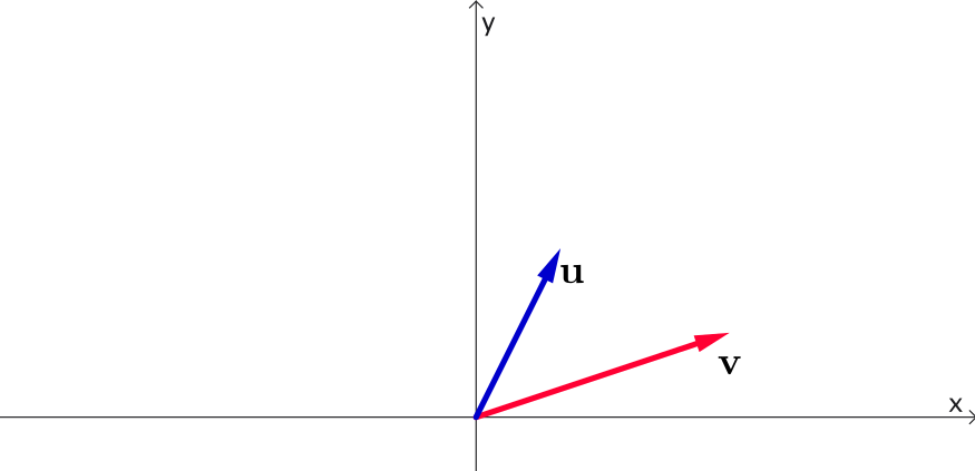
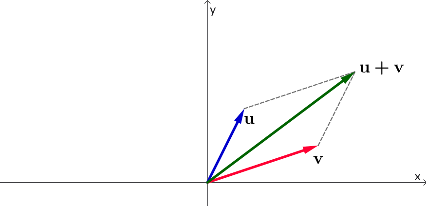
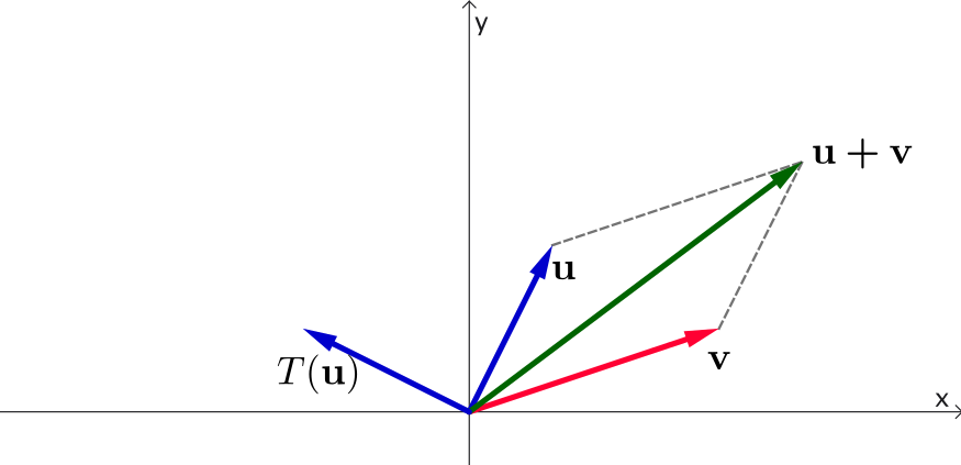
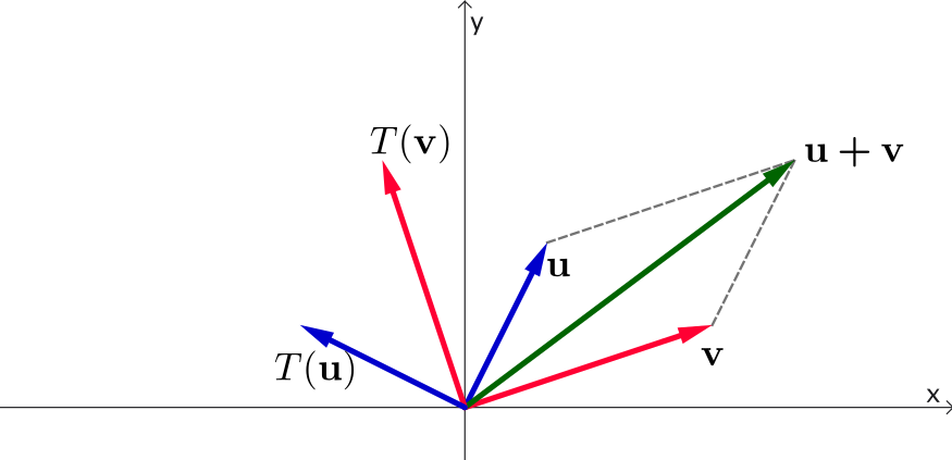
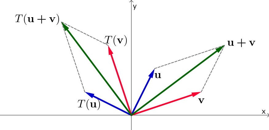
Geometrically, we can see that the diagonal of the sum vector parallelogram rotates along with its components. In other words,
$T(\mathbf{u}+\mathbf{v}) = T(\mathbf{u}) + T(\mathbf{v})$
Example of a Linear Transformation (2)
Similarly, for scaling a vector by a scalar constant $\alpha$, under the same $90^{\circ}$ anti-clockwise rotation:
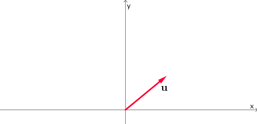
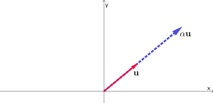
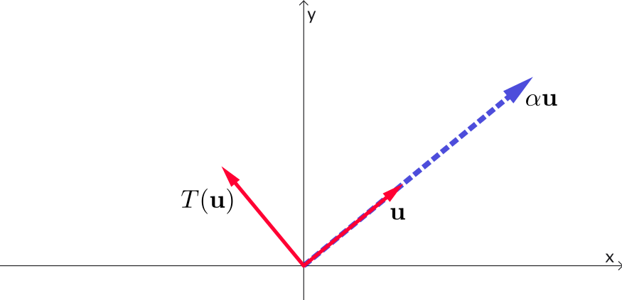
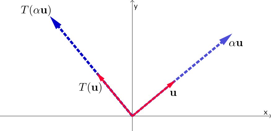
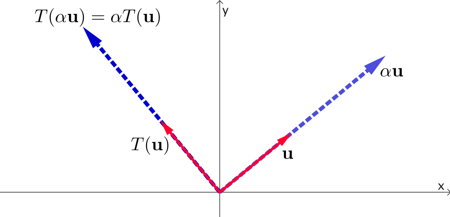
Therefore, $T(\alpha \mathbf{u}) = \alpha T(\mathbf{u})$ holds true.
A Mapping That is NOT a Linear Transformation
$T:\mathbb{R}^2 \rightarrow \mathbb{R}^2$ given by $T\begin{pmatrix} x \\ y \end{pmatrix} = \begin{pmatrix} x + 1 \\ y \end{pmatrix}$
Let's test with a counterexample. Say $\mathbf{u} = \begin{pmatrix} 2 \\ 1 \end{pmatrix}$ and $\mathbf{v} = \begin{pmatrix} 1 \\ 1 \end{pmatrix}$:
$\mathbf{u}+\mathbf{v} = \begin{pmatrix} 3 \\ 2 \end{pmatrix} $ $ \implies T(\mathbf{u}+\mathbf{v}) = \begin{pmatrix} 4 \\ 2 \end{pmatrix} $
But computing them individually yields:
$ T(\mathbf{u}) = \begin{pmatrix} 3 \\ 1 \end{pmatrix}, \quad T(\mathbf{v}) = \begin{pmatrix} 2 \\ 1 \end{pmatrix} $ $ \implies T(\mathbf{u}) + T(\mathbf{v}) = \begin{pmatrix} 5 \\ 2 \end{pmatrix} $
Since $T(\mathbf{u}) + T(\mathbf{v}) \neq T(\mathbf{u}+\mathbf{v})$, it is not a linear transformation.
Note: You can disprove linearity with a single counterexample. However, to prove a mapping is a linear transformation, you must show it holds in general.
Linear Transformations
📝 Practice examples
- Show that the following mapping $T:\mathbb{R}^2 \mapsto \mathbb{R}^2$ is not linear: $$T\begin{pmatrix} x_1 \\ x_2 \end{pmatrix} = \begin{pmatrix} x_2 \\ x_1 - 1 \end{pmatrix}$$
- Determine whether the transformation $T:\mathbb{R}^2 \mapsto \mathbb{R}^3$ is linear: $$T\begin{pmatrix} x_1 \\ x_2 \end{pmatrix} = \begin{pmatrix} x_1 \\ x_2 \\ x_1^2 + x_2^2 \end{pmatrix}$$
📝 Practice example 1
$T:\mathbb{R}^2 \rightarrow \mathbb{R}^2$ given by $ T\begin{pmatrix}x_1\\x_2\end{pmatrix} = \begin{pmatrix} x_2\\ x_1-1 \end{pmatrix} $
Let's test with a counterexample. Say $ \mathbf{u}= \begin{pmatrix}1\\0\end{pmatrix}, \;\; \mathbf{v}= \begin{pmatrix}0\\1\end{pmatrix}. $
$ \mathbf{u}+\mathbf{v} = \begin{pmatrix}1\\1\end{pmatrix} $ $ \implies T(\mathbf{u}+\mathbf{v}) = \begin{pmatrix}1\\0\end{pmatrix} $
But computing them individually yields:
$ T(\mathbf{u}) = \begin{pmatrix}0\\0\end{pmatrix}, \;\; T(\mathbf{v}) = \begin{pmatrix}1\\-1\end{pmatrix} $ $ \implies T(\mathbf{u})+T(\mathbf{v}) = \begin{pmatrix}1\\-1\end{pmatrix} $
Since $ T(\mathbf{u}+\mathbf{v}) \neq T(\mathbf{u})+T(\mathbf{v}), $ the mapping is not a linear transformation.
Note: A single counterexample is enough to disprove linearity.
📝 Practice example 2
$T:\mathbb{R}^2 \rightarrow \mathbb{R}^3$ given by $ T\begin{pmatrix}x_1\\x_2\end{pmatrix} = \begin{pmatrix} x_1\\ x_2\\ x_1^2+x_2^2 \end{pmatrix} $
Let's test the additivity property. Take $ \mathbf{u}= \begin{pmatrix}1\\0\end{pmatrix}, \; \mathbf{v}= \begin{pmatrix}0\\1\end{pmatrix}. $
$ \mathbf{u}+\mathbf{v} = \begin{pmatrix}1\\1\end{pmatrix} $ $ \implies T(\mathbf{u}+\mathbf{v}) = \begin{pmatrix}1\\1\\2\end{pmatrix} $
Individual computation gives: $ T(\mathbf{u}) = \begin{pmatrix}1\\0\\1\end{pmatrix}, \; T(\mathbf{v}) = \begin{pmatrix}0\\1\\1\end{pmatrix} $ $ \implies T(\mathbf{u})+T(\mathbf{v}) = \begin{pmatrix}1\\1\\2\end{pmatrix} $
So, for these vectors, $ T(\mathbf{u}+\mathbf{v}) = T(\mathbf{u})+T(\mathbf{v}). $
Practice example 2
$T:\mathbb{R}^2 \rightarrow \mathbb{R}^3$ given by $ T\begin{pmatrix}x_1\\x_2\end{pmatrix} = \begin{pmatrix} x_1\\ x_2\\ x_1^2+x_2^2 \end{pmatrix} $
However, this does not prove that $T$ is linear.
The mapping is still not a linear transformation.
Why?
We must also verify the homogeneity property,
$
T(c\mathbf{x}) = c\,T(\mathbf{x}),
$
which this mapping does not satisfy because of the quadratic term
$x_1^2+x_2^2$.
Proving a Mapping is a Linear Transformation
Consider another transformation on $\mathbb{R}^2$ given by $T(\mathbf{v}) = 3\mathbf{v}$. We check the core properties to confirm if $T$ is linear.
(a) Check whether $T(\mathbf{u}+\mathbf{v}) = T(\mathbf{u}) + T(\mathbf{v})$
Let $\mathbf{u} = \begin{pmatrix} u_1 \\ u_2 \end{pmatrix}$ and $\mathbf{v} = \begin{pmatrix} v_1 \\ v_2 \end{pmatrix}$, meaning $\mathbf{u}+\mathbf{v} = \begin{pmatrix} u_1 + v_1 \\ u_2 + v_2 \end{pmatrix}$:
$ T(\mathbf{u}+\mathbf{v}) = T\begin{pmatrix} u_1 + v_1 \\ u_2 + v_2 \end{pmatrix} $ $ = 3\begin{pmatrix} u_1 + v_1 \\ u_2 + v_2 \end{pmatrix} $ $ = \begin{pmatrix} 3u_1 + 3v_1 \\ 3u_2 + 3v_2 \end{pmatrix} $
$ \quad = 3\begin{pmatrix} u_1 \\ u_2 \end{pmatrix} + 3\begin{pmatrix} v_1 \\ v_2 \end{pmatrix} $ $ = T(\mathbf{u}) + T(\mathbf{v})\quad $ ✅
Proving a Mapping is a Linear Transformation
Consider another transformation on $\mathbb{R}^2$ given by $T(\mathbf{v}) = 3\mathbf{v}$. We check the core properties to confirm if $T$ is linear.
(a) Check whether $T(\mathbf{u}+\mathbf{v}) = T(\mathbf{u}) + T(\mathbf{v})$
(b) Check whether $T(\alpha \mathbf{u}) = \alpha T(\mathbf{u})$
Using the same mapping $T(\mathbf{v}) = 3\mathbf{v}$ with an arbitrary scalar $\alpha \in \mathbb{R}$:
$ T(\alpha \mathbf{u}) = T\begin{pmatrix} \alpha u_1 \\ \alpha u_2 \end{pmatrix} $ $ = 3\begin{pmatrix} \alpha u_1 \\ \alpha u_2 \end{pmatrix} $ $ = \alpha \left[ 3\begin{pmatrix} u_1 \\ u_2 \end{pmatrix} \right] $ $ = \alpha T(\mathbf{u})\quad $ ✅
Proving a Mapping is a Linear Transformation
Consider another transformation on $\mathbb{R}^2$ given by $T(\mathbf{v}) = 3\mathbf{v}$. We check the core properties to confirm if $T$ is linear.
(a) Check whether $T(\mathbf{u}+\mathbf{v}) = T(\mathbf{u}) + T(\mathbf{v})$
(b) Check whether $T(\alpha \mathbf{u}) = \alpha T(\mathbf{u})$
Both rules are satisfied!
So $T(\mathbf{v}) = 3\mathbf{v}$ is rigorously proven to be a linear transformation!
Using the Alternate Definition
Consider the mapping from $\mathbb{R}^2$ to $\mathbb{R}^3$ given by:
$ T\begin{pmatrix} x_1 \\ x_2 \end{pmatrix} = \left(x_2, x_1, x_1 + x_2\right)^T = \begin{pmatrix} x_2 \\ x_1 \\ x_1 + x_2 \end{pmatrix}$
We will show that this is linear using the single consolidated criteria: $$T\left(\alpha \mathbf{u} + \beta \mathbf{v}\right) = \alpha T(\mathbf{u}) + \beta T(\mathbf{v}).$$
Let $\mathbf{u} = \begin{pmatrix} u_1 \\ u_2 \end{pmatrix}$ and $\mathbf{v} = \begin{pmatrix} v_1 \\ v_2 \end{pmatrix}$. Then $\;\alpha \mathbf{u} + \beta \mathbf{v} = \begin{pmatrix} \alpha u_1 + \beta v_1 \\ \alpha u_2 + \beta v_2 \end{pmatrix}.$
Using the Alternate Definition
Consider the mapping from $\mathbb{R}^2$ to $\mathbb{R}^3$ given by:
$ T\begin{pmatrix} x_1 \\ x_2 \end{pmatrix} = \left(x_2, x_1, x_1 + x_2\right)^T = \begin{pmatrix} x_2 \\ x_1 \\ x_1 + x_2 \end{pmatrix}$
Thus $\alpha \mathbf{u} + \beta \mathbf{v} = \begin{pmatrix} \alpha u_1 + \beta v_1 \\ \alpha u_2 + \beta v_2 \end{pmatrix}$. Applying the rules of mapping $T$ gives:
$T(\alpha \mathbf{u} + \beta \mathbf{v}) = \begin{pmatrix} \alpha u_2 + \beta v_2 \\ \alpha u_1 + \beta v_1 \\ (\alpha u_1 + \beta v_1) + (\alpha u_2 + \beta v_2) \end{pmatrix}$ $= \begin{pmatrix} \alpha u_2 \\ \alpha u_1 \\ \alpha u_1 + \alpha u_2 \end{pmatrix} + \begin{pmatrix} \beta v_2 \\ \beta v_1 \\ \beta v_1 + \beta v_2 \end{pmatrix}$
$= \alpha \begin{pmatrix} u_2 \\ u_1 \\ u_1 + u_2 \end{pmatrix} + \beta \begin{pmatrix} v_2 \\ v_1 \\ v_1 + v_2 \end{pmatrix}$ $= \alpha T(\mathbf{u}) + \beta T(\mathbf{v})$
📝 Exercises
- Show that the following transformation $T : \mathbb{R}^2 \rightarrow \mathbb{R}^2$ is linear: $$T\begin{pmatrix} x_1 \\ x_2 \end{pmatrix} = \begin{pmatrix} 2x_1 \\ x_2 \end{pmatrix}$$
- Show that $T : \mathbb{R}^2 \rightarrow \mathbb{R}^2$ given by the following mapping is a linear transformation: $$T\begin{pmatrix} x_1 \\ x_2 \end{pmatrix} = \begin{pmatrix} x_2 \\ 3x_1 \end{pmatrix}$$
Solution to Exercise 1
1. Consider $ T:\mathbb{R}^2\rightarrow\mathbb{R}^2, \quad T\begin{pmatrix}x_1\\x_2\end{pmatrix} = \begin{pmatrix} 2x_1\\ x_2 \end{pmatrix}. $
To prove that $T$ is linear, show that $ T(\alpha\mathbf{u}+\beta\mathbf{v}) = \alpha T(\mathbf{u}) + \beta T(\mathbf{v}) $ for all vectors $\mathbf{u},\mathbf{v}$ and scalars $\alpha,\beta$.
Let $ \mathbf{u}= \begin{pmatrix}u_1\\u_2\end{pmatrix}, \; \mathbf{v}= \begin{pmatrix}v_1\\v_2\end{pmatrix}. $ Then
$ T(\alpha\mathbf{u}+\beta\mathbf{v}) = T\!\left( \begin{pmatrix} \alpha u_1+\beta v_1\\ \alpha u_2+\beta v_2 \end{pmatrix} \right) $ $ = \begin{pmatrix} 2(\alpha u_1+\beta v_1)\\ \alpha u_2+\beta v_2 \end{pmatrix} $
$ = \alpha \begin{pmatrix} 2u_1\\ u_2 \end{pmatrix} + \beta \begin{pmatrix} 2v_1\\ v_2 \end{pmatrix} $ $ = \alpha T(\mathbf{u}) + \beta T(\mathbf{v}). $
Since this holds for all $\mathbf{u},\mathbf{v}\in\mathbb{R}^2$ and all $\alpha,\beta\in\mathbb{R}$, $T$ is a linear transformation.
If $T(\mathbf{x})$ is a Linear Transformation, $T(\mathbf{0}) = \mathbf{0}$
Theorem: For any linear transformation $T(\mathbf{x})$, $T(\mathbf{0}) = \mathbf{0}$.
Proof Outline
-
From the definition of a linear transformation,
$\alpha T(\mathbf{0}) $ $ = T(\alpha \mathbf{0})$ $= T(\mathbf{0})$
for any scalar constant $\alpha$.
- If $\alpha T(\mathbf{0}) = T(\mathbf{0})$ holds true for all $\alpha$, then $T(\mathbf{0})$ must equal $\mathbf{0}$.
Corollary: If $T(\mathbf{0}) \neq \mathbf{0}$ for any given mapping structure, it cannot be a linear transformation.
A Linear Transformation That is Not on $\mathbb{R}^n$
Consider the definite integral operator $I : C[a, b] \rightarrow \mathbb{R}$ defined by: $$I\left(f\right) = \ds \int_{a}^{b} f(t) \,dt$$
(where $C[a, b]$ represents the set of all continuous functions on the interval $[a, b]$).
Let's show that $I\left(\alpha f + \beta g\right) = \alpha I(f) + \beta I(g)$, for functions $f, g \in C[a, b]$ and constants $\alpha, \beta \in \mathbb{R}$:
$\ds I\left(\alpha f + \beta g\right) $ $\ds = \int_{a}^{b} \big[\alpha f(t) + \beta g(t)\big] \, dt$ $\ds = \alpha \int_{a}^{b} f(t) \, dt + \beta \int_{a}^{b} g(t) \, dt \quad \quad\;\; $
$\quad \ds = \alpha I(f) + \beta I(g) \quad \text{(using calculus rules of integration)}$
Thus, this calculus integration operator is a linear transformation.
Another Linear Transformation That is Not on $\mathbb{R}^n$
Consider the derivative operator $T = \dfrac{d}{dx}$ mapping $P_2 \rightarrow P_1$, where $P_n$ is the vector space of polynomials of degree $n$ or less.
$T$ acts on a polynomial to take its derivative:
$T\left(c_1 + c_2x + c_3x^2\right) $ $= \dfrac{d}{dx}\left(c_1 + c_2x + c_3x^2\right) $ $= c_2 + 2c_3x$
📝 Exercise for you:
Can you prove that this derivative operator is a linear transformation?
Hint: Set up two arbitrary general polynomials within $P_2$, say $p_1 = a_1 + a_2x + a_3x^2$ and $p_2 = c_1 + c_2x + c_3x^2$, then test the criteria.
Matrix Representation
Revisiting our prior example where $T\begin{pmatrix} x_1 \\ x_2 \end{pmatrix} = \begin{pmatrix} x_2 \\ x_1 \\ x_1 + x_2 \end{pmatrix}.$
Let's define matrix $A\,$ as $\,A = \begin{pmatrix} 0 & 1 \\ 1 & 0 \\ 1 & 1 \end{pmatrix}.$ We can rewrite the transformation cleanly as matrix multiplication:
$T(\mathbf{x}) = \begin{pmatrix} x_2 \\ x_1 \\ x_1 + x_2 \end{pmatrix}$ $= \begin{pmatrix} 0 & 1 \\ 1 & 0 \\ 1 & 1 \end{pmatrix} \begin{pmatrix} x_1 \\ x_2 \end{pmatrix} $ $ = A\mathbf{x}$
It is true in general that any operation defined by $T(\mathbf{x}) = A\mathbf{x}$ forms a linear transformation.
Matrix Representation Theorem
The Standard Basis
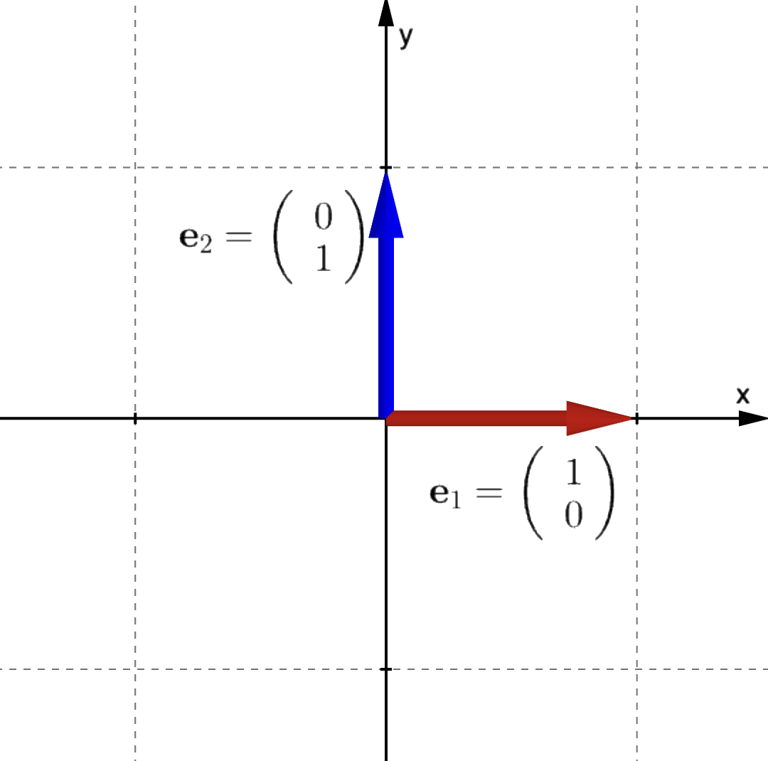
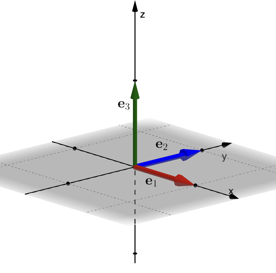
The standard basis in $\mathbb{R}^n$ is the collection of mutually orthogonal unit vectors:
$\mathbf{e}_1 = \begin{pmatrix} 1 \\ 0 \\ \vdots \\ 0 \end{pmatrix}, \quad \mathbf{e}_2 = \begin{pmatrix} 0 \\ 1 \\ \vdots \\ 0 \end{pmatrix}, \quad \dots, \quad \mathbf{e}_n = \begin{pmatrix} 0 \\ 0 \\ \vdots \\ 1 \end{pmatrix}$

Matrix Representation Theorem
The Standard Basis
|
For $\mathbb R^2$ $\mathbf{e}_1 = \begin{pmatrix} 1 \\ 0 \end{pmatrix}, \;\; \mathbf{e}_2 = \begin{pmatrix} 0 \\ 1 \end{pmatrix}$ |
|
Matrix Representation Theorem
The Standard Basis
|
For $\mathbb R^3$ $\mathbf{e}_1 = \begin{pmatrix} 1 \\ 0 \\ 0\end{pmatrix}, \;\; \mathbf{e}_2 = \begin{pmatrix} 0 \\ 1 \\ 0 \end{pmatrix}, $ $\mathbf{e}_3 = \begin{pmatrix} 0 \\ 0 \\ 1 \end{pmatrix}$ |
|
Matrix Representation Theorem
Theorem: If $T$ is a linear transformation mapping from $\mathbb{R}^n$ into $\mathbb{R}^m$, there exists a unique $m \times n$ matrix $A$ such that $T(\mathbf{x}) = A\mathbf{x}$ for all $\mathbf{x} \in \mathbb{R}^n$.
Crucially, the $j$-th column vector of $A$ is found by transforming the standard basis element $\mathbf{e}_j$. That is, $\,\mathbf{a}_j = T(\mathbf{e}_j)$ for $j = 1, 2, \dots, n$.
Proof Outline:
Let $A = \begin{pmatrix} \mathbf{a}_1 & \mathbf{a}_2 & \dots & \mathbf{a}_n \end{pmatrix}$ where $\mathbf{a}_j = T(\mathbf{e}_j)$.
Any vector $\mathbf{x} \in \mathbb{R}^n$ can be broken down as: $\mathbf{x} = x_1\mathbf{e}_1 + x_2\mathbf{e}_2 + \dots + x_n\mathbf{e}_n$
$\implies T(\mathbf{x}) = x_1 T(\mathbf{e}_1) + x_2 T(\mathbf{e}_2) + \dots + x_n T(\mathbf{e}_n) \quad \text{(by linearity properties)}$
$\implies T(\mathbf{x}) = x_1\mathbf{a}_1 + x_2\mathbf{a}_2 + \dots + x_n\mathbf{a}_n$
Matrix Representation Theorem
Theorem: If $T$ is a linear transformation mapping from $\mathbb{R}^n$ into $\mathbb{R}^m$, there exists a unique $m \times n$ matrix $A$ such that $T(\mathbf{x}) = A\mathbf{x}$ for all $\mathbf{x} \in \mathbb{R}^n$.
Proof Outline:
$\implies T(\mathbf{x}) = x_1\mathbf{a}_1 + x_2\mathbf{a}_2 + \dots + x_n\mathbf{a}_n$
Expanding the linear combination $T(\mathbf{x}) = x_1\mathbf{a}_1 + x_2\mathbf{a}_2 + \dots + x_n\mathbf{a}_n$ into component forms:
$T(\mathbf x)= x_1 \begin{pmatrix} a_{11} \\ a_{21} \\ \vdots \\ a_{m1} \end{pmatrix} + x_2 \begin{pmatrix} a_{12} \\ a_{22} \\ \vdots \\ a_{m2} \end{pmatrix} + \dots + x_n \begin{pmatrix} a_{1n} \\ a_{2n} \\ \vdots \\ a_{mn} \end{pmatrix}$ $= \begin{pmatrix} a_{11} & a_{12} & \dots & a_{1n} \\ a_{21} & a_{22} & \dots & a_{2n} \\ \vdots & \vdots & \ddots & \vdots \\ a_{m1} & a_{m2} & \dots & a_{mn} \end{pmatrix} \begin{pmatrix} x_1 \\ x_2 \\ \vdots \\ x_n \end{pmatrix} $ $= A\mathbf{x}$
This is exactly equivalent to the standard definition of matrix multiplication.
Matrix Representation - Example
Find the matrix representation for the linear mapping $T: \mathbb{R}^3 \rightarrow \mathbb{R}^2$ given by
$T(\mathbf{x}) = (x_1 + x_2, x_2 + x_3)^T$ where $\mathbf{x} = (x_1, x_2, x_3)^T$.
We evaluate $T$ for each element of the standard basis of $\mathbb{R}^3$:
$T(\mathbf{e}_1) = T\begin{pmatrix} 1 \\ 0 \\ 0 \end{pmatrix} $ $ = \begin{pmatrix} 1+0 \\ 0+0 \end{pmatrix} $ $= \begin{pmatrix} 1 \\ 0 \end{pmatrix},\quad$ $T(\mathbf{e}_2) = T\begin{pmatrix} 0 \\ 1 \\ 0 \end{pmatrix} $ $ = \begin{pmatrix} 0+1 \\ 1+0 \end{pmatrix} $ $ = \begin{pmatrix} 1 \\ 1 \end{pmatrix},$
$T(\mathbf{e}_3) = T\begin{pmatrix} 0 \\ 0 \\ 1 \end{pmatrix} $ $ = \begin{pmatrix} 0+0 \\ 0+1 \end{pmatrix} $ $ = \begin{pmatrix} 0 \\ 1 \end{pmatrix} $
Stacking these results into columns yields the transformation matrix $A$:
$A = \begin{pmatrix} 1 & 1 & 0 \\ 0 & 1 & 1 \end{pmatrix}$
2D Geometric Transformations with Matrices
Geometric Interpretation
Suppose you are given the transformation matrix $A = \begin{pmatrix} 1 & 0
\\ 0 & -1
\end{pmatrix}$.
How would you describe the operation $T(\mathbf{v}) = A\mathbf{v}$ geometrically?
Use a general vector $\mathbf{v} = \begin{pmatrix} v_1 \\ v_2 \end{pmatrix}$ and calculate the output:
$T(\mathbf{v}) = A\mathbf{v} $ $ = \begin{pmatrix} 1 & 0 \\ 0 & -1 \end{pmatrix}\begin{pmatrix} v_1 \\ v_2 \end{pmatrix} $ $= \begin{pmatrix} v_1 \\ -v_2 \end{pmatrix} $
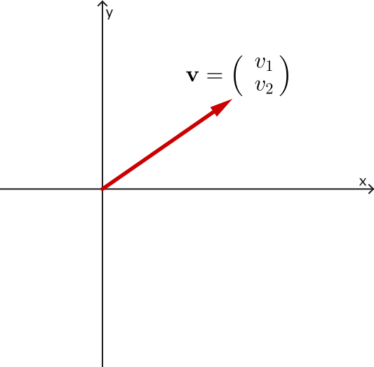
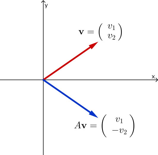
Conclusion: This transformation reflects points across the horizontal $x$-axis.
2D Geometric Transformations with Matrices
Geometric Interpretation
How would you describe the operation $T(\mathbf{v}) = A\mathbf{v}$ geometrically?
|
$T(\mathbf{v}) = A\mathbf{v} = \begin{pmatrix} 1 & 0 \\ 0 & -1 \end{pmatrix}\begin{pmatrix} v_1 \\ v_2 \end{pmatrix} $ $ \qquad = \begin{pmatrix} v_1 \\ -v_2 \end{pmatrix} $ 👉 Reflection in the $x$-axis |
|
2D Geometric Transformations with Matrices
Reflection in the $x$-axis
When coordinates are reflected across the $x$-axis, the mappings translate as follows:
$\begin{pmatrix} x \\ y \end{pmatrix} \mapsto \begin{pmatrix} x \\ -y \end{pmatrix}$
Tracing the transformation of standard basis vectors:
$ \mathbf{e}_1 = \begin{pmatrix} 1 \\ 0 \end{pmatrix} \mapsto \begin{pmatrix} 1 \\ 0 \end{pmatrix} \quad $ $ \text{and} \quad \mathbf{e}_2 = \begin{pmatrix} 0 \\ 1 \end{pmatrix} \mapsto \begin{pmatrix} 0 \\ -1 \end{pmatrix} $
Assembling these vectors into columns gives the transformation matrix:
$$A = \begin{pmatrix} 1 & 0 \\ 0 & -1 \end{pmatrix}$$2D Geometric Transformations with Matrices
Reflection in the $y$-axis
When coordinates are instead reflected across the vertical $y$-axis, the mappings change to:
$\begin{pmatrix} x \\ y \end{pmatrix} \mapsto \begin{pmatrix} -x \\ y \end{pmatrix}$
Tracing the transformation of standard basis vectors:
$ \mathbf{e}_1 = \begin{pmatrix} 1 \\ 0 \end{pmatrix} \mapsto \begin{pmatrix} -1 \\ 0 \end{pmatrix} \quad $ $ \text{and} \quad \mathbf{e}_2 = \begin{pmatrix} 0 \\ 1 \end{pmatrix} \mapsto \begin{pmatrix} 0 \\ 1 \end{pmatrix} $
Grouping columns together produces the canonical matrix:
$$A = \begin{pmatrix} -1 & 0 \\ 0 & 1 \end{pmatrix}$$2D Geometric Transformations with Matrices
Reflection in the $y$-axis
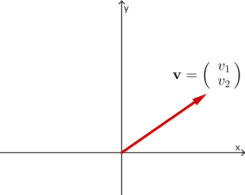
Geometric interpretation
|
$T(\mathbf{v}) = A\mathbf{v} = \begin{pmatrix} -1 & 0 \\ 0 & 1 \end{pmatrix}\begin{pmatrix} v_1 \\ v_2 \end{pmatrix} $ $ \qquad = \begin{pmatrix} -v_1 \\ v_2 \end{pmatrix} $ 👉 Reflection in the $y$-axis |
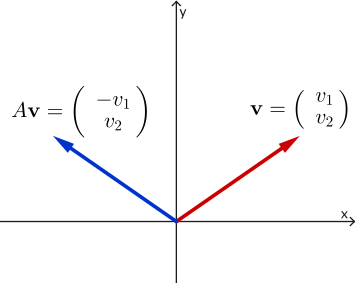
|
2D Geometric Transformations with Matrices
Rotation through an Angle $\theta$
To rotate the standard 2D axes counterclockwise by a generic angle $\theta$:
- The vector $\mathbf{e}_1 = \begin{pmatrix} 1 \\ 0 \end{pmatrix}$ moves onto unit circle coords: $\begin{pmatrix} \cos\theta \\ \sin\theta \end{pmatrix}$
- The vector $\mathbf{e}_2 = \begin{pmatrix} 0 \\ 1 \end{pmatrix}$ moves onto perpendicular coords: $\begin{pmatrix} -\sin\theta \\ \cos\theta \end{pmatrix}$
Combining these columns yields the fundamental 2D rotation matrix:
$$A = \begin{pmatrix} \cos\theta & -\sin\theta \\ \sin\theta & \cos\theta \end{pmatrix}$$2D Geometric Transformations with Matrices
Rotation through an Angle $\theta$
For instance, a pure $90^{\circ}$ anti-clockwise rotation sets $\theta = \dfrac{\pi}{2}$. Thus
$A = \begin{pmatrix} \cos \dfrac{\pi}{2} & -\sin \dfrac{\pi}{2} \\ \sin \dfrac{\pi}{2} & \cos \dfrac{\pi}{2} \end{pmatrix} $ $= \begin{pmatrix} 0 & -1 \\ 1 & 0 \end{pmatrix} $ $ \Ra \begin{pmatrix} 0 & -1 \\ 1 & 0 \end{pmatrix}\begin{pmatrix} x \\ y \end{pmatrix} = \begin{pmatrix} -y \\ x \end{pmatrix}$
Note: For numerical computations, it is more common to use radians instead of degrees.
Matrices as Linear transformations
Application: Computer graphics and Animations

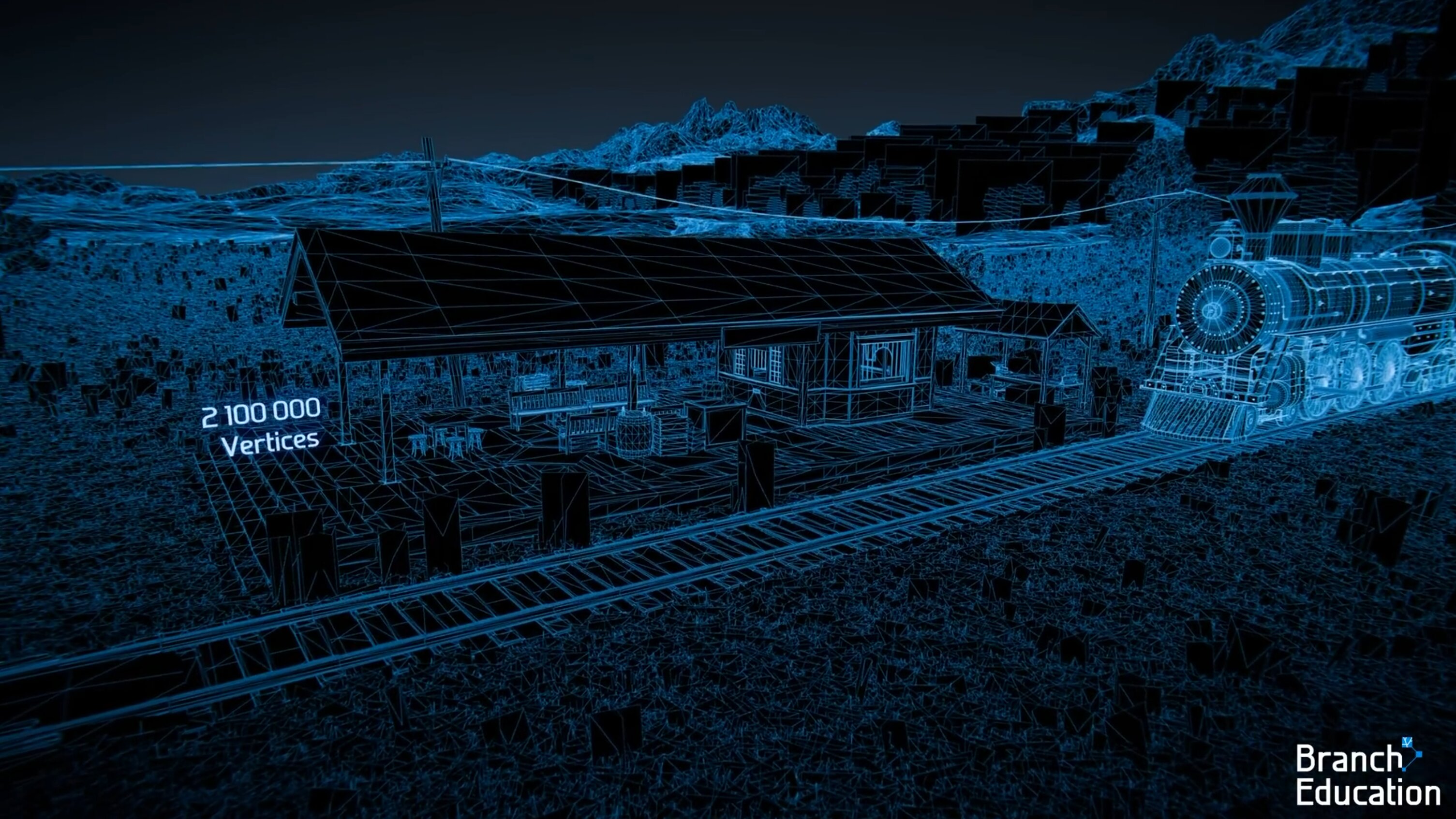



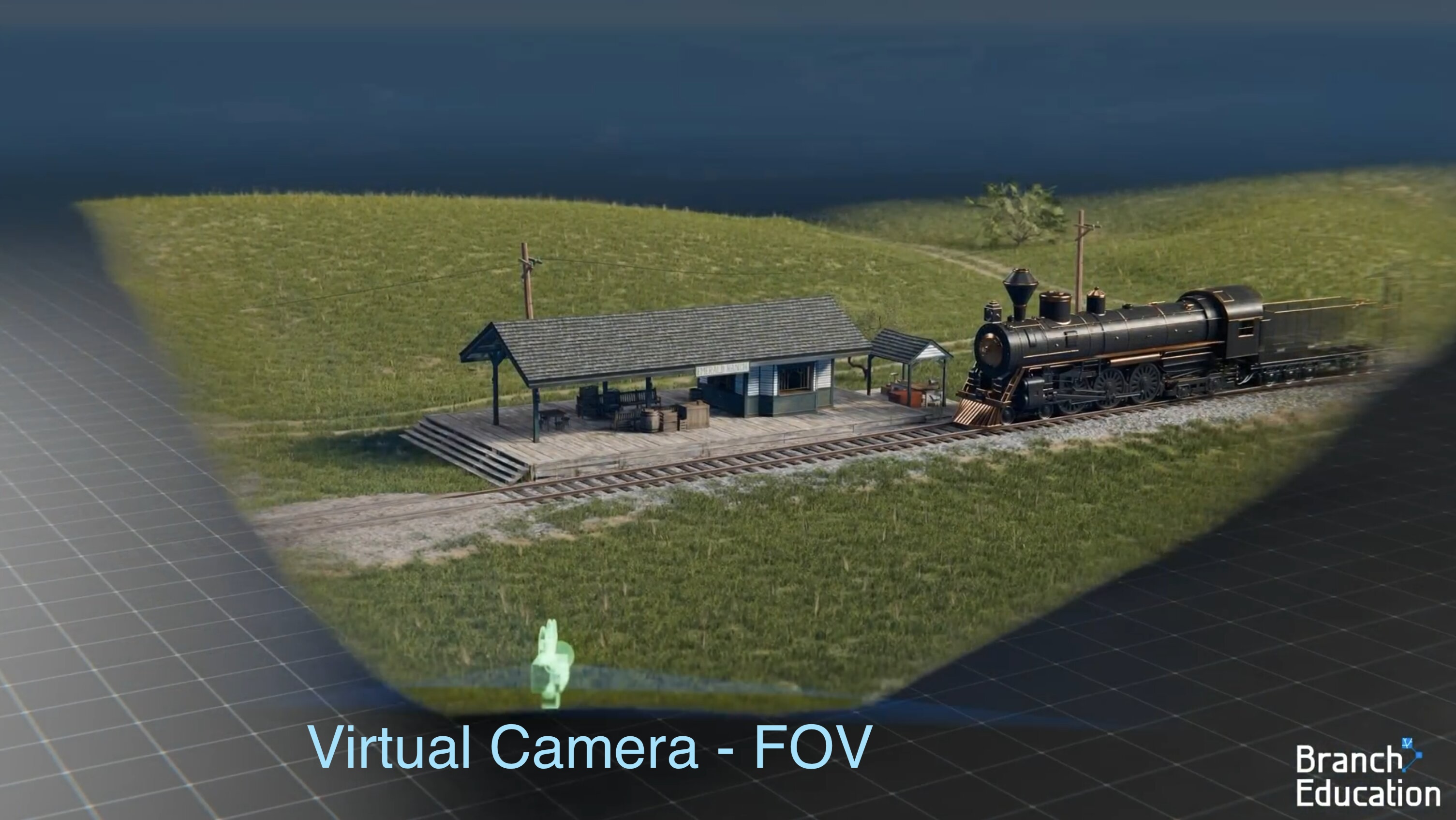
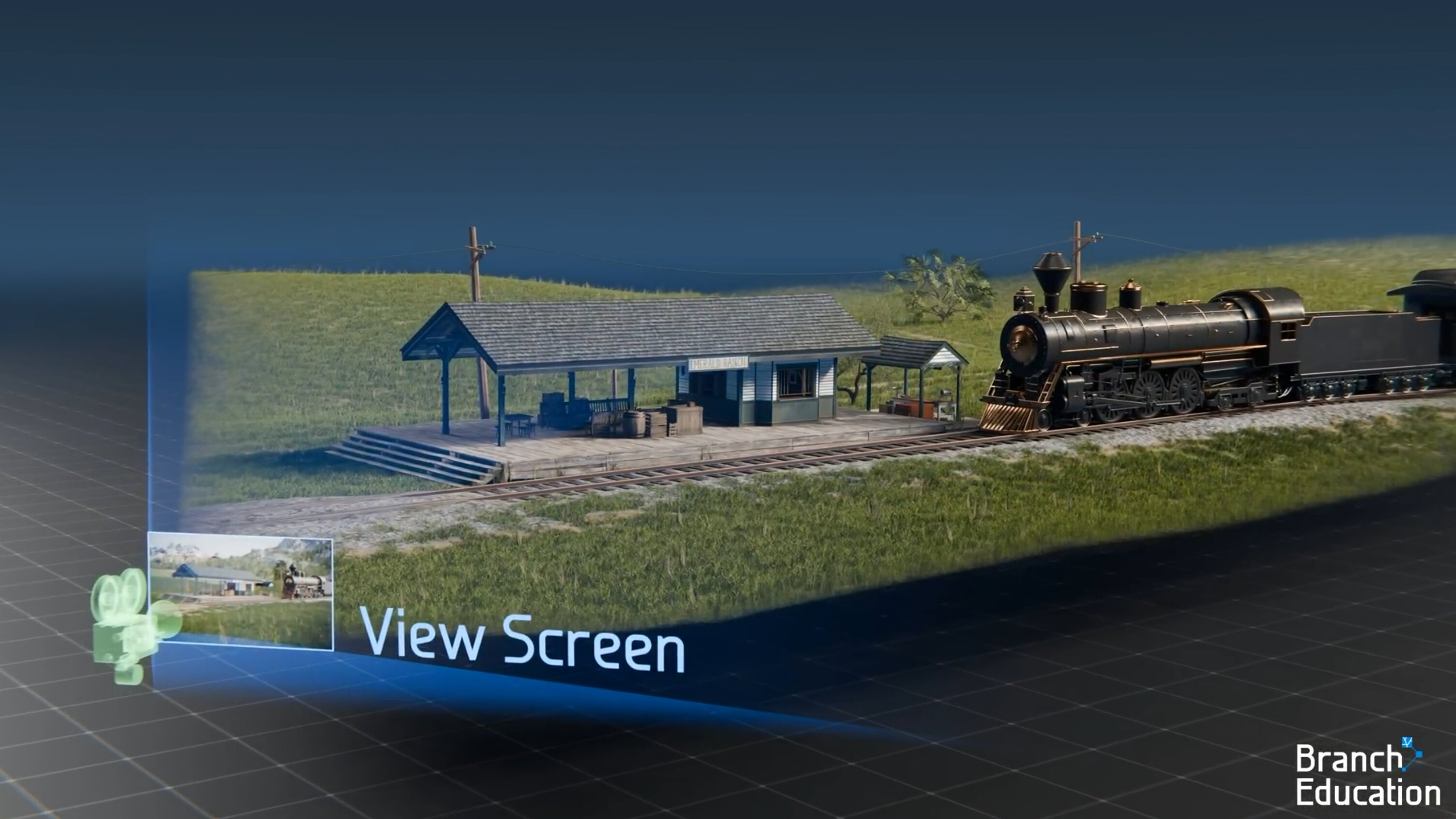
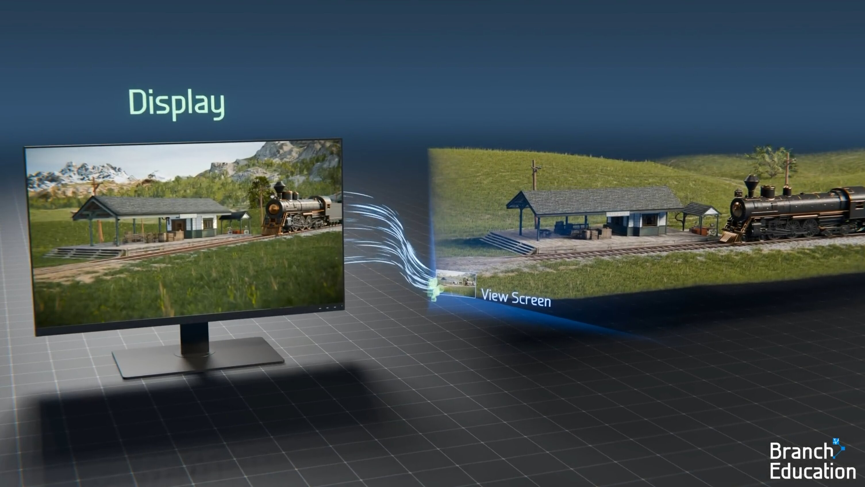
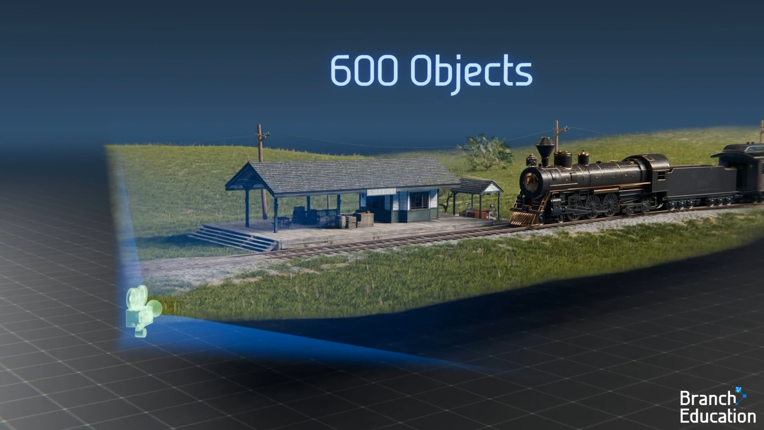
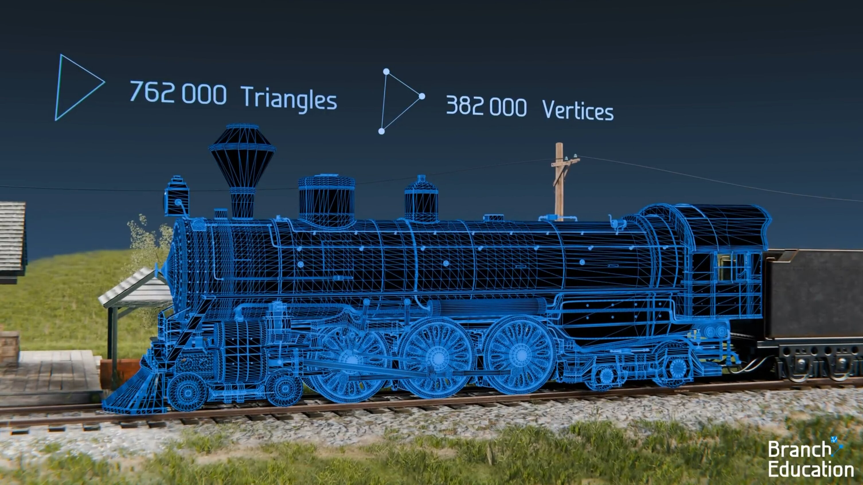
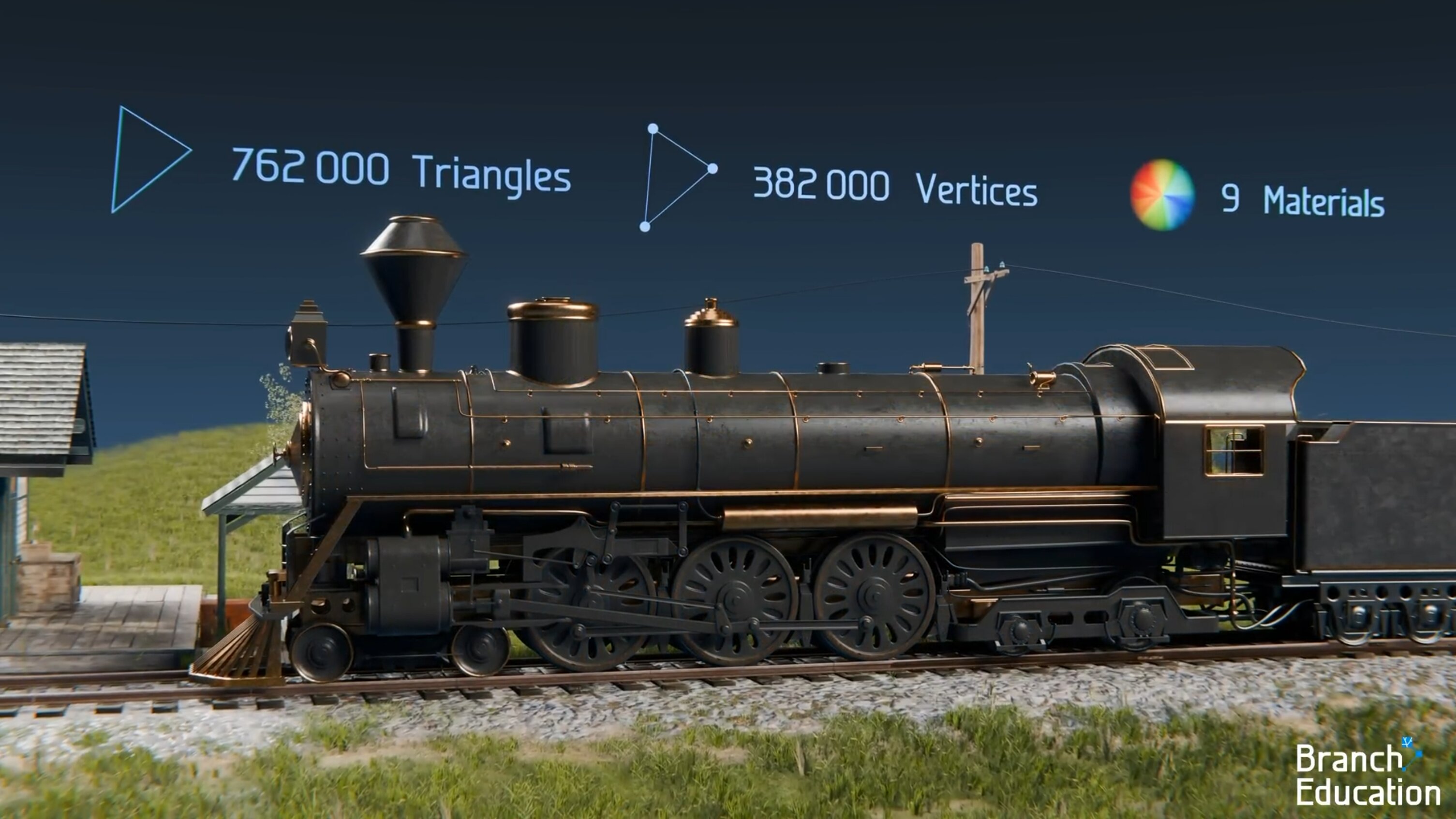
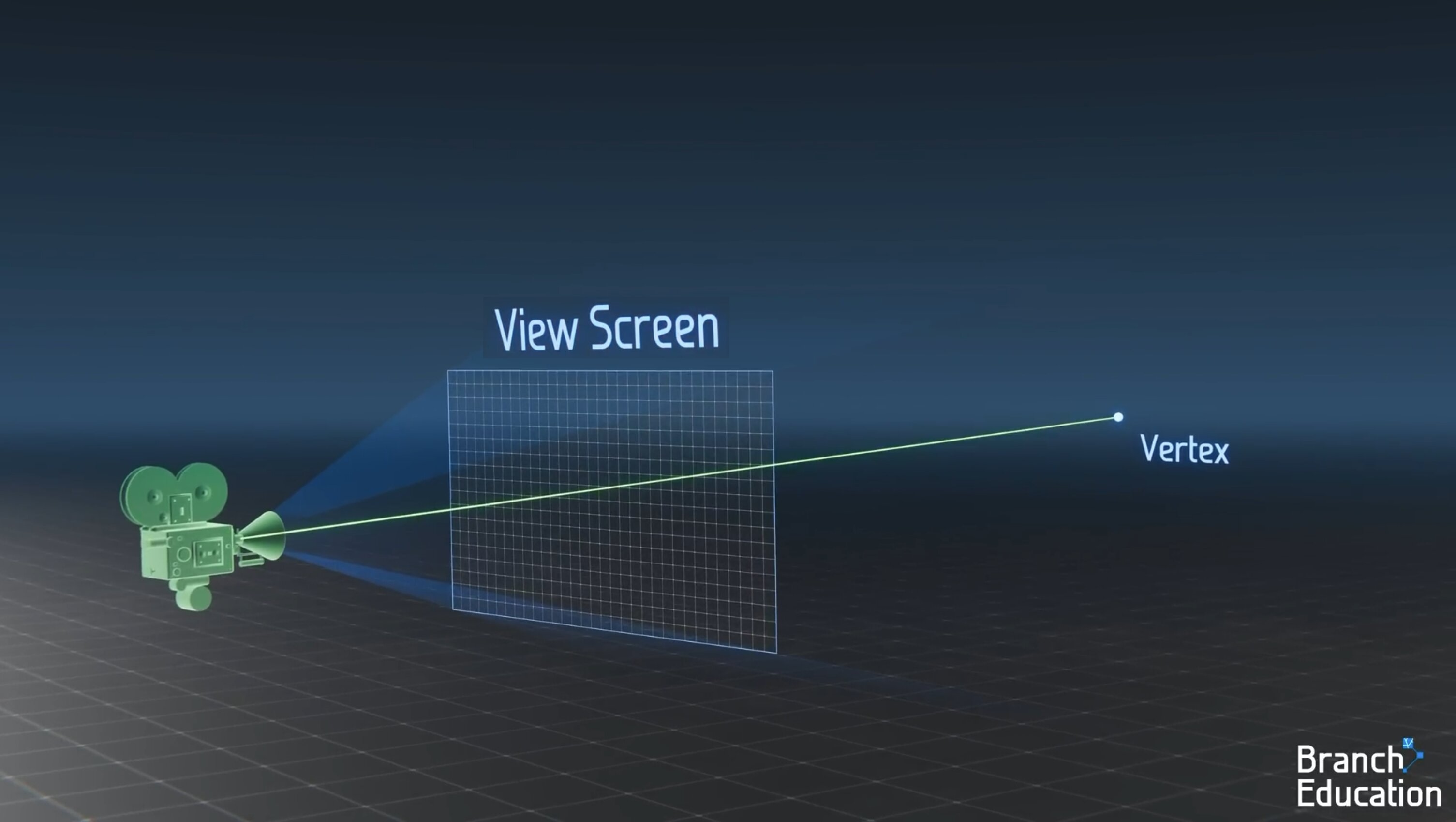
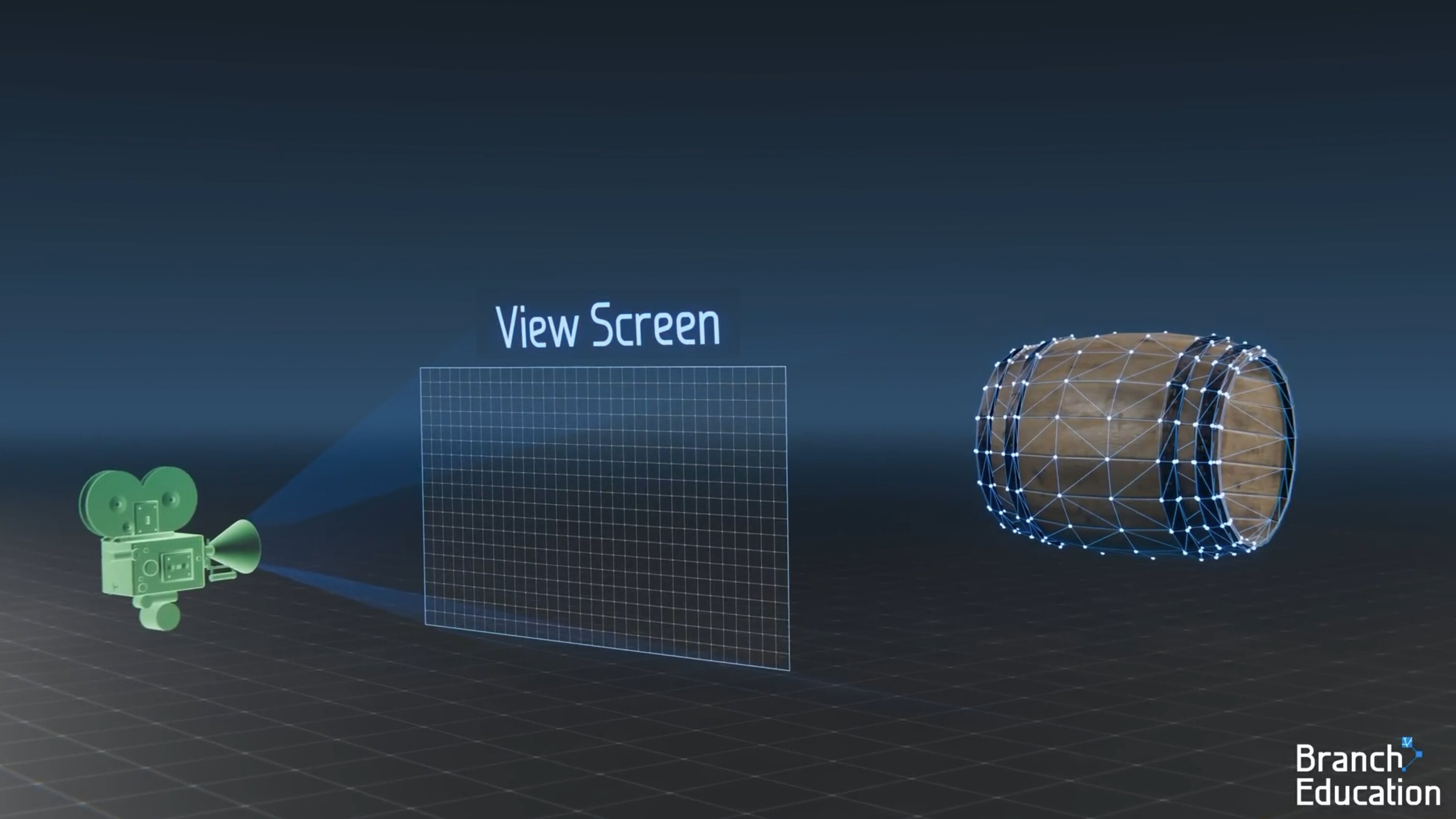
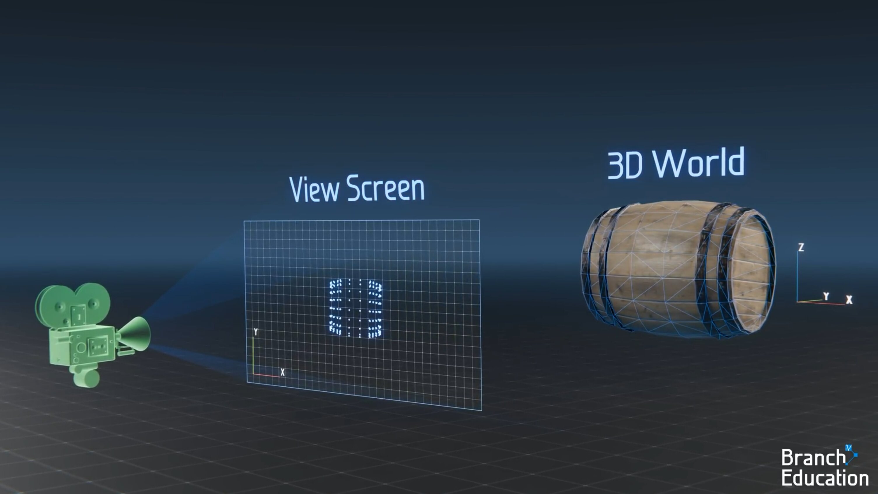
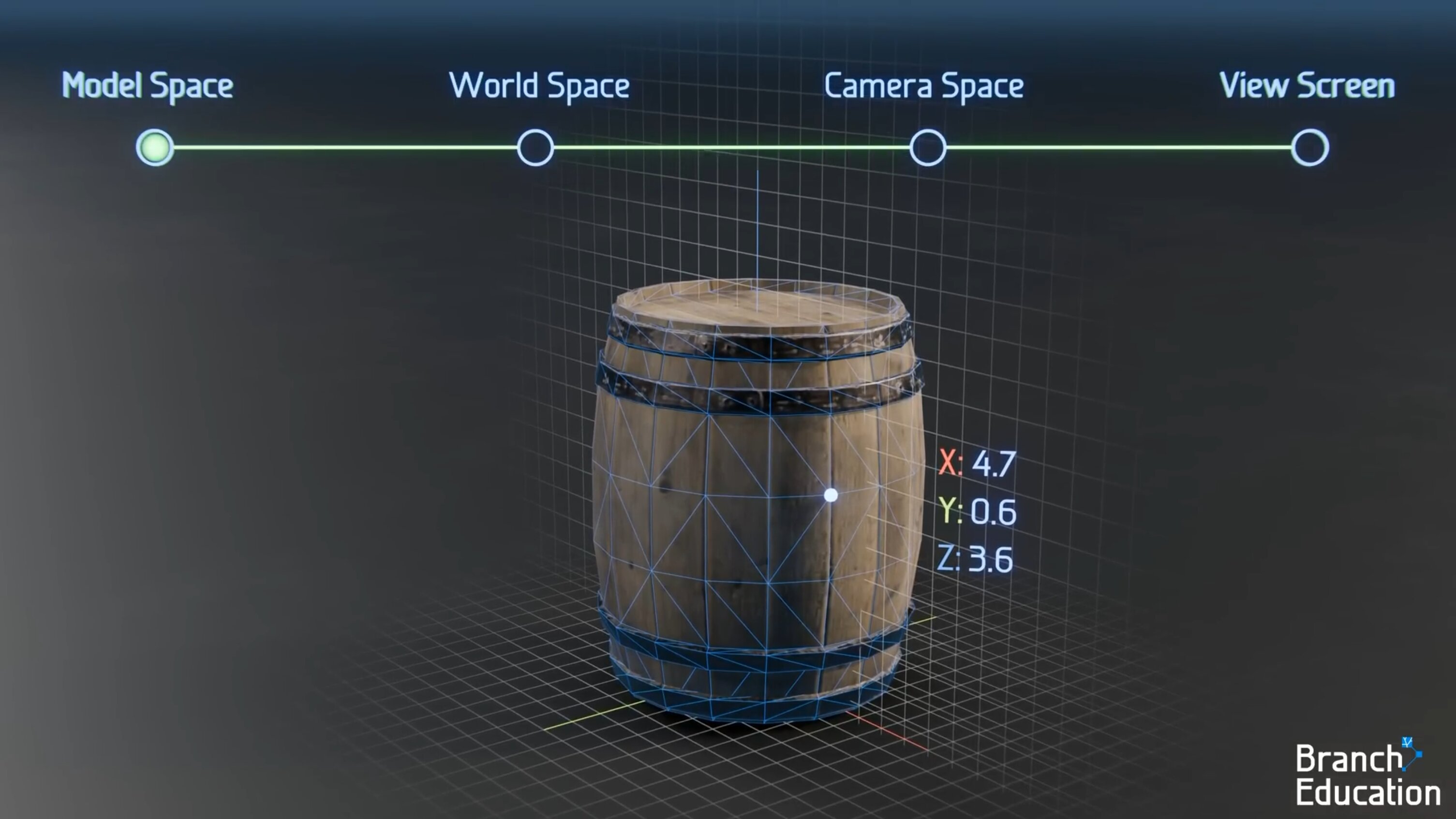
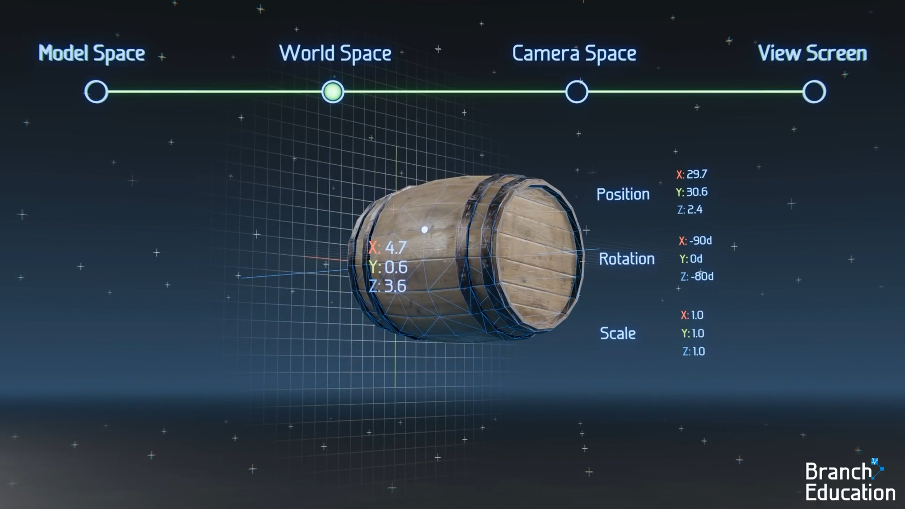
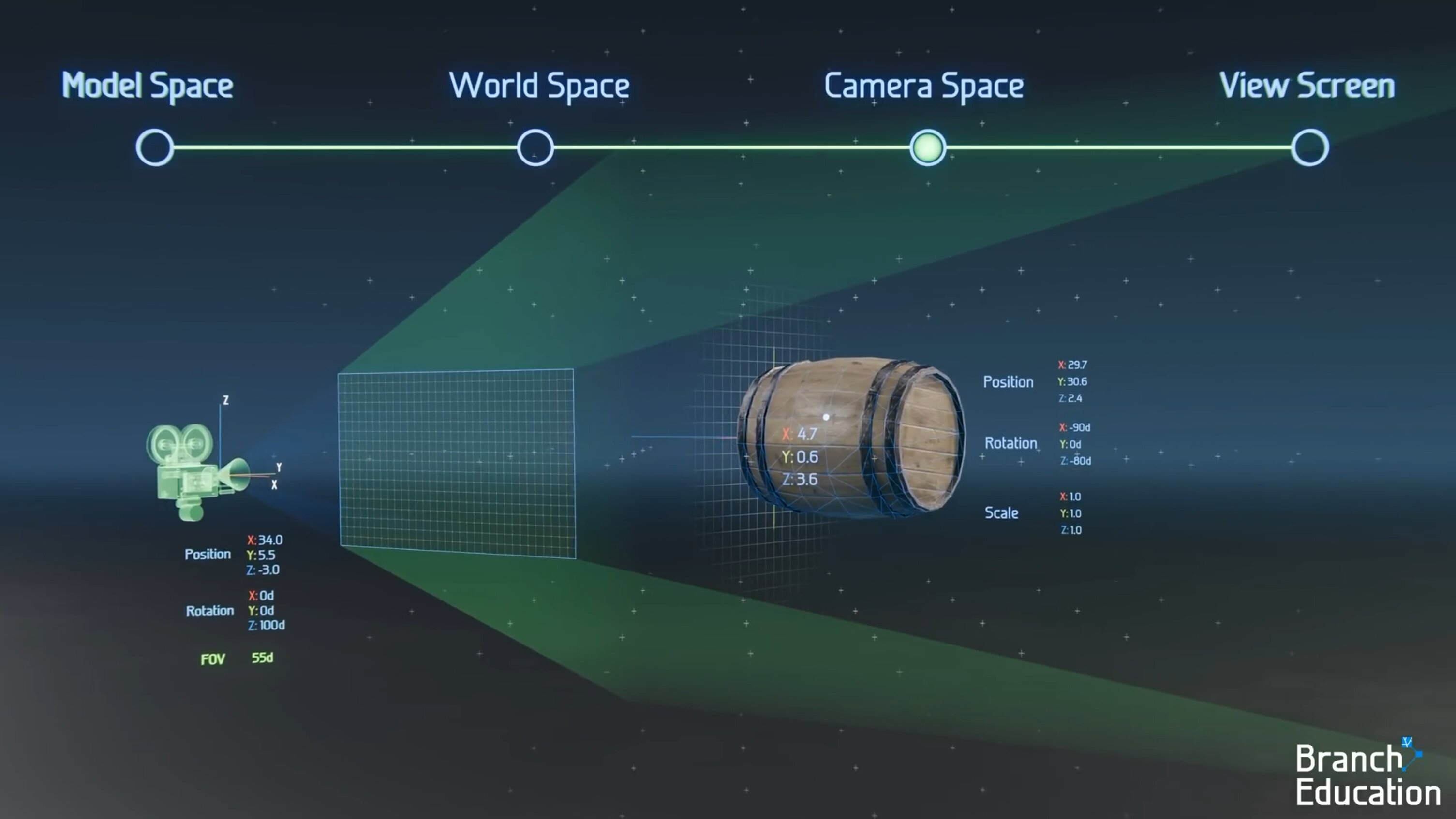
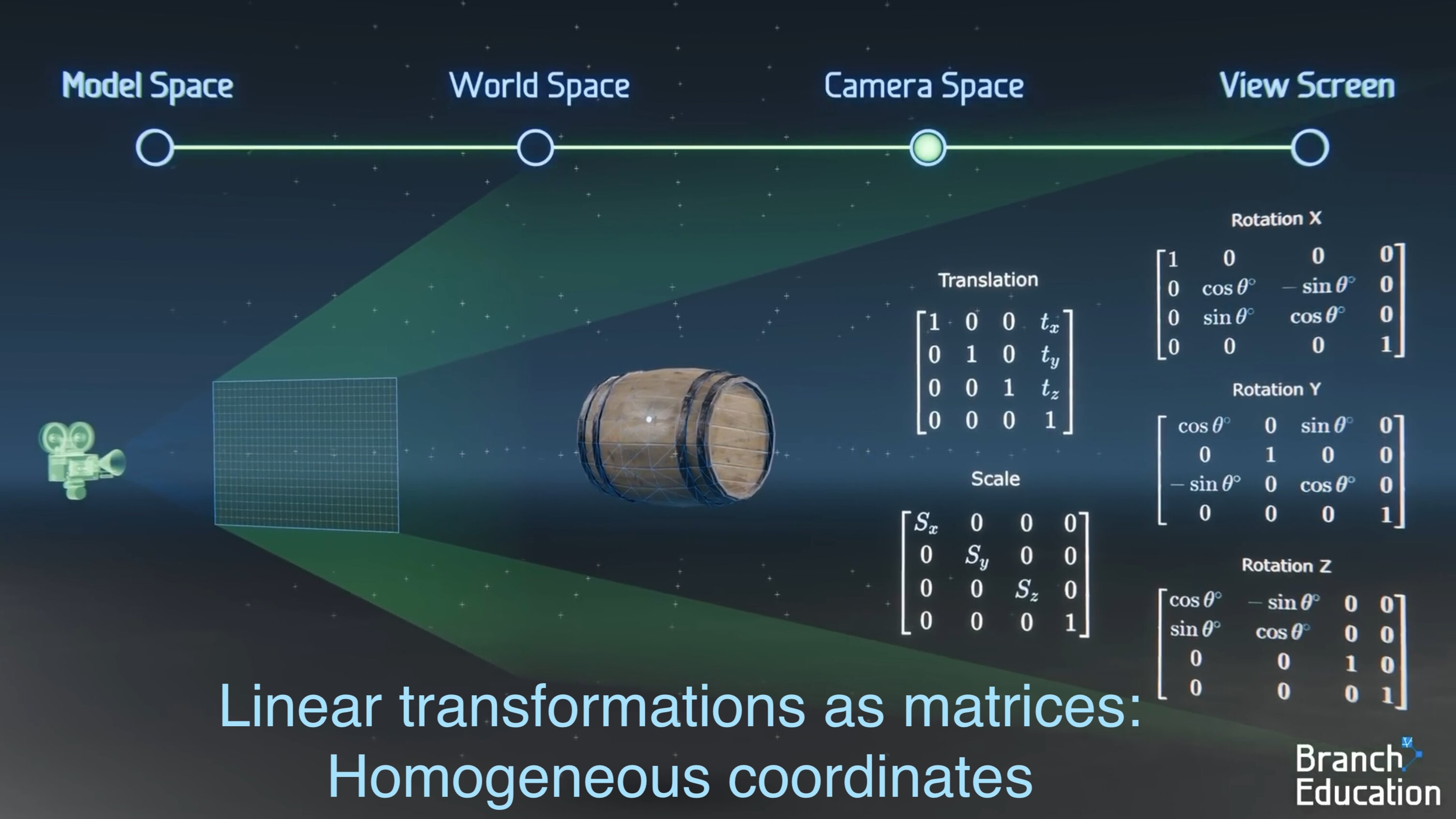
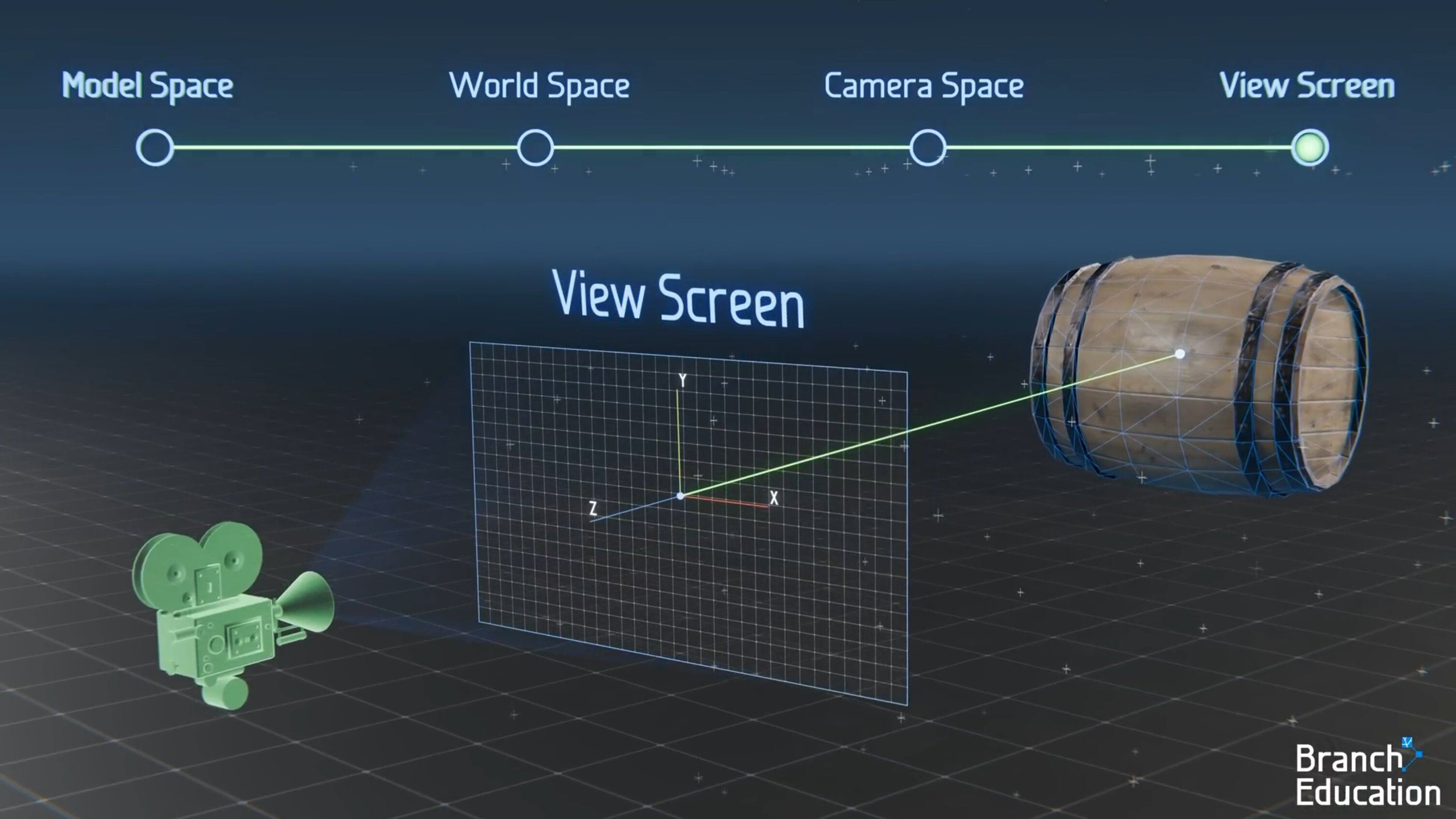
Application: Computer graphics and Animations
Source: 🎥 Branch Education - How do Video Game Graphics Work?
www.youtube.com/@BranchEducation

2D Geometric Transformations with Matrices
📝 Practice Example
- Find the standard matrix representation of a
transformation $T$ that:
- Rotates each vector $\mathbf{x} \in \mathbb{R}^2$ by $60^{\circ}$ in the anti-clockwise direction.
- Reflects each vector $\mathbf{x} \in \mathbb{R}^2$ across the $y$-axis.
- Reflects each vector $\mathbf{x} \in \mathbb{R}^2$ across the $y$-axis and then rotates it $60^{\circ}$ anti-clockwise.
- Doubles the length of each vector $\mathbf{x} \in \mathbb{R}^2$ and then rotates it $30^{\circ}$ clockwise.
Inverse Linear Transformations
Theorem: Let $T:\mathbb R^n \to \mathbb R^n$ be a linear transformation with matrix $A.$ Then the inverse transformation $T^{-1}$ exists if and only if $\det(A)\neq 0.$ Furthermore, $T^{-1}:\mathbb R^n \to \mathbb R^n$ is a linear transformation with matrix $A^{-1}.$
Example: If $T:\mathbb R^3 \to \mathbb R^3$ has a matrix \[A = \left( \begin{array}{ccc} 2 & 3 & 1\\ -1 & 2 & 3\\ 4 & 2 & 6\\ \end{array} \right), \]
then \(T^{-1}\) exists since \(\det(A) = 63\) \(\neq 0.\) This means that $A$ is invertible and $A^{-1}$ exists. Therefore $T^{-1}$ exists and is given by $T^{-1}(\mathbf x) = A^{-1}\mathbf x.$
Inverse Linear Transformations
Theorem: Let $T:\mathbb R^n \to \mathbb R^n$ be a linear transformation with matrix $A.$ Then the inverse transformation $T^{-1}$ exists if and only if $\det(A)\neq 0.$ Furthermore, $T^{-1}:\mathbb R^n \to \mathbb R^n$ is a linear transformation with matrix $A^{-1}.$
Example: To determine the inverse of $A$ we can apply the Gauss-Jordan elimination:
$ \left( \begin{array}{ccc|ccc} 2 & 3 & 1 & 1 & 0 & 0 \\ -1 & 2 & 3& 0 & 1 & 0 \\ 4 & 1 & 6 & 0 & 0 & 1 \\ \end{array} \right) $
$ \left( \begin{array}{ccc|ccc} 1 & \frac{3}{2} & \frac{1}{2} & \frac{1}{2} & 0 & 0 \\ -1 & 2 & 3& 0 & 1 & 0 \\ 4 & 1 & 6 & 0 & 0 & 1 \\ \end{array} \right) \begin{array}{c} \frac{1}{2}R1 \\ \\ \\ \end{array} $
$ \left( \begin{array}{ccc|ccc} 1 & \frac{3}{2} & \frac{1}{2} & \frac{1}{2} & 0 & 0 \\ 0 & \frac{7}{2} & \frac{7}{2} & \frac{1}{2} & 1 & 0 \\ 4 & 1 & 6 & 0 & 0 & 1 \\ \end{array} \right) \begin{array}{c} \\ R2 +R1 \\ \\ \end{array} $
$ \left( \begin{array}{ccc|ccc} 1 & \frac32 & \frac12 & \frac12&0&0\\ 0&1&1&\frac17&\frac27&0\\ 4&1&6&0&0&1 \end{array} \right) \begin{array}{c} \\ \frac27R2\\ \\ \end{array} $
$ \left( \begin{array}{ccc|ccc} 1&0&-1&\frac27&-\frac37&0\\ 0&1&1&\frac17&\frac27&0\\ 4&1&6&0&0&1 \end{array} \right) \begin{array}{c} R1-\frac32R2\\ \\ \\ \end{array} $
$ \left( \begin{array}{ccc|ccc} 1&0&-1&\frac27&-\frac37&0\\ 0&1&1&\frac17&\frac27&0\\ 0&1&10&-\frac87&\frac{12}{7}&1 \end{array} \right) \begin{array}{c} \\ \\ R3-4R1 \end{array} $
$ \left( \begin{array}{ccc|ccc} 1&0&-1&\frac27&-\frac37&0\\ 0&1&1&\frac17&\frac27&0\\ 0&0&9&-\frac97&\frac{10}{7}&1 \end{array} \right) \begin{array}{c} \\ \\ R3-R2 \end{array} $
$ \left( \begin{array}{ccc|ccc} 1&0&-1&\frac27&-\frac37&0\\ 0&1&1&\frac17&\frac27&0\\ 0&0&1&-\frac17&\frac{10}{63}&\frac19 \end{array} \right) \begin{array}{c} \\ \\ \frac19R3 \end{array} $
$ \left( \begin{array}{ccc|ccc} 1&0&0&\frac17&-\frac{17}{63}&\frac19\\ 0&1&1&\frac17&\frac27&0\\ 0&0&1&-\frac17&\frac{10}{63}&\frac19 \end{array} \right) \begin{array}{c} R1+R3\\ \\ \\ \end{array} $
$ \left( \begin{array}{ccc|ccc} 1&0&0&\frac17&-\frac{17}{63}&\frac19\\ 0&1&0&\frac27&\frac{8}{63}&-\frac19\\ 0&0&1&-\frac17&\frac{10}{63}&\frac19 \end{array} \right) \begin{array}{c} \\ R2-R3\\ \\ \end{array} $
$ A^{-1}= \left( \begin{array}{ccc} \frac17&-\frac{17}{63}&\frac19\\ \frac27&\frac{8}{63}&-\frac19\\ -\frac17&\frac{10}{63}&\frac19 \end{array} \right) $
So \(\, T^{-1}\left(\mathbf x^T\right) \) \( =T^{-1}\left( \left(x_1, x_2, x_3\right)^T\right) \)
\( = \big( \frac{1}{7} x_1 - \frac{17}{63}x_2+\frac{1}{9}x_3, \frac{2}{7} x_1 + \frac{8}{63}x_2-\frac{1}{9}x_3, -\frac{1}{7} x_1 + \frac{10}{63}x_2+\frac{1}{9}x_3 \big)^T \)
Composition of Linear Transformations
Theorem:Let $T_{1}:\mathbb{R}^{n}\rightarrow\mathbb{R}^{m}$ and $T_{2}:\mathbb{R}^{m}\rightarrow\mathbb{R}^{p}$ be linear transformations with matrices $A$ and $B$, respectively. Then the composition transformation $T_{2}\circ T_{1}:\mathbb{R}^{n}\rightarrow\mathbb{R}^{p}$ is a linear transformation with matrix $BA$.
Proof Outline
$(T_{2}\circ T_{1})(\mathbf{x}) $ $ = T_{2}(T_{1}(\mathbf{x}))$ $= T_{2}(A\mathbf{x})$ $= B(A\mathbf{x})$ $= (BA)\mathbf{x}$.
Composition of Linear Transformations
Example of a Product Transformation
Reflect each vector $\mathbf{x}\in\mathbb{R}^2$ across the $y$-axis and then rotate it $60^\circ$ anti-clockwise.
$$ R_y=\begin{pmatrix}-1&0\\0&1\end{pmatrix}, \qquad R_{60}= \begin{pmatrix} \frac12&-\frac{\sqrt3}{2}\\ \frac{\sqrt3}{2}&\frac12 \end{pmatrix}. $$
Since the reflection is applied first, $ T\rightarrow R_{60}R_y. $
$ R_{60}R_y = \begin{pmatrix} \frac12&-\frac{\sqrt3}{2}\\ \frac{\sqrt3}{2}&\frac12 \end{pmatrix} \begin{pmatrix} -1&0\\ 0&1 \end{pmatrix} $ $= \begin{pmatrix} -\frac12&-\frac{\sqrt3}{2}\\ -\frac{\sqrt3}{2}&\frac12 \end{pmatrix}.$
Thus, the matrix representing the composition is $ \begin{pmatrix} -\frac12&-\frac{\sqrt3}{2}\\ -\frac{\sqrt3}{2}&\frac12 \end{pmatrix}. $
Composition of Linear Transformations
Example of a Product Transformation
Double the length of each vector $\mathbf{x}\in\mathbb{R}^2$ and then rotate it $30^\circ$ clockwise.
$$ S= \begin{pmatrix} 2&0\\ 0&2 \end{pmatrix}, \qquad R_{-30}= \begin{pmatrix} \frac{\sqrt3}{2}&\frac12\\ -\frac12&\frac{\sqrt3}{2} \end{pmatrix}. $$
Since the scaling is applied first, $ T\rightarrow R_{-30}S. $
$ R_{-30}S = \begin{pmatrix} \frac{\sqrt3}{2}&\frac12\\ -\frac12&\frac{\sqrt3}{2} \end{pmatrix} \begin{pmatrix} 2&0\\ 0&2 \end{pmatrix} $ $ = \begin{pmatrix} \sqrt3&1\\ -1&\sqrt3 \end{pmatrix}.$
Thus, the matrix representing the composition is $ \begin{pmatrix} \sqrt3&1\\ -1&\sqrt3 \end{pmatrix}. $
Composition of Linear Transformations
A More General Example of a Product Transformation
Let
$T_{1}:M_n\big(\mathbb R\big)\to M_n\big(\mathbb R\big)\;$ and $\;T_{2}:M_n\big(\mathbb R\big)\to \mathbb R$
be linear transformations defined as
$T_1 \left(A\right) = A + A^T\;$ and $\;T_2\left(A\right) = \text{tr}\left(A\right),$
where $M_n\big(\mathbb R\big)$ is the set of real $n\times n$ matrices and $\text{tr}(A)$ is the trace of $A$ (i.e. the sum of elements on the main diagonal).
Then $T_{2}\circ T_{1}:M_n\big(\mathbb R\big)\rightarrow\mathbb{R}$ is defined by:
$ \big(T_{2}\circ T_{1}\big)(A) $ $=T_{2}\big(T_{1}(A)\big)$ $=T_{2}\left(A+A^{T}\right)$ $=\text{tr}\left(A+A^{T}\right)$
Composition of Linear Transformations
A More General Example of a Product Transformation
Let
$T_{1}:M_n\big(\mathbb R\big)\to M_n\big(\mathbb R\big)\;$ and $\;T_{2}:M_n\big(\mathbb R\big)\to \mathbb R$
be linear transformations defined as
$T_1 \left(A\right) = A + A^T\;$ and $\;T_2\left(A\right) = \text{tr}\left(A\right),$
$ \big(T_{2}\circ T_{1}\big)(A) $ $=T_{2}\big(T_{1}(A)\big)$ $=T_{2}\left(A+A^{T}\right)$ $=\text{tr}\left(A+A^{T}\right)$
For example, if $A=\begin{pmatrix}2&-1\\ -3&6\end{pmatrix}$ then:
$T_{1}(A)=A+A^{T}$, $=\begin{pmatrix}4&-4\\ -4&12\end{pmatrix}$, so that $T_{2}\big(T_{1}(A)\big)$ $=\text{tr}\begin{pmatrix}4&-4\\ -4&12\end{pmatrix}$ $=16$.
Summary of Properties of Linear Transformations
- For any linear transformation $T$ from $\mathbb{R}^{n}$ to $\mathbb{R}^{m}$ we can find an $m\times n$ matrix $A$ so that $T(\mathbf{v})=A\mathbf{v}$.
- If the transformation is invertible, the inverse transformation has the matrix $A^{-1}$.
- The composition of two transformations $T_{1}(\mathbf{v})=A_{1}\mathbf{v}$ and $T_{2}(\mathbf{v})=A_{2}\mathbf{v}$ is the product matrix $A_{2}A_{1}$.
Summary of Linear Transformations Section
- Examples of linear transformations
- Demonstration that some mappings are not linear transformations
- How to show that a mapping is a linear transformation
- Matrix representation of a linear transformation using the standard basis
- Rotation and reflection matrices (2D)
- Application Example: Simple computer graphics
- Inverse and Composite linear transformations